Binding Site Comparison Benchmarks - II - Binding sites on the similar proteins

Introduction

The previous post of this series established a first protocol on how to identify & cluster the ATP binding site of the N-terminal domain of human HSP90 alpha. It can be generalized to other proteins as well but to keep it simple I’ll continue this series on a single protein for now and generalize at a later stage.

In this second post we’ll gradually extend the dataset with ATP binding sites of proteins that are very similar to the human HSP90 alpha.

What is similar?

One can adopt several ways to assess the similarity between proteins. Here I’ll use a commonly understood and accepted sequence local similarity on the N-terminal domain. I’ll further assess the binding site residue conservation in detail. So at this stage of the dataset creation I’ll focus on things I’d expect to be found as very very similar to the human HSP90 alpha N-terminal domain when doing a pocket comparison. The Rognan lab discussed this topic in more than one paper. Feel free to check out Kellenberger, Schalon, and Rognan (2008) and Eguida and Rognan (2022) for more details.

Things to keep in mind

Again I’ll track all things that I left aside or important approximations I made. They’ll be tracked as side-note and depending on the outcome of the whole exercise I’ll come back to them at a later stage.

Things to keep in mind

• listing goes here

Methods & Results

Identify similar sequences

In order to identify similar sequences one usually would do just a simple blast. Unfortunately, things are a bit trickier. First of all, we are currently looking only at the N-terminal domain of HSP90 (around 230 amino acids). The full human HSP90 alpha protein has 732 amino acids. So, shall we search for globally similar sequences? or smaller regions?

The N-terminal part is considered to be a domain, so structured on itself. There are numerous structure resolution papers that show that, Sreeramulu et al. (2009) is just one of them, as an example here, where only the N-terminal domain of HSP90 is amplified, produced & resolved.

We could even go further and use only the range of amino acids that are involved in the ATP binding site. In the case of a small domain like this one here that might not be required, but for large domains it might be of interest to focus on the binding site only. In this example this would mean start at the glutamate 47 and go up to the valine 186 (+ maybe a few flanking residues)

For the sake of simplicity I’ll take the whole N-terminal domain (amino acids 9-236), corresponding to the first region of HS90A_HUMAN in the UniProt database.

The blast mess

Now let’s try to set up a first blast search. We want to find PDB structures containing a resolved portion of the domain of interest (or similar). There are unfortunately thousands of services allowing to do that, and as usual they don’t give the same results. One important factor is to search against an up to date version of the RCSB PDB. The only service I found that clearly states what release of the PDB is being used is NCBI blastp page.

I don’t want to reinvent the wheel or install blast locally etc, so here I’ll use the biotite (Kunzmann and Hamacher (2018)) integration of the NCBI blast service.

import biotite.sequence.io.fasta as fasta
import biotite.application.blast as blast
from biotite.sequence import ProteinSequence
import urllib
import io 
import pickle

uniprotcode="P07900"
start=9
end=236
url="https://rest.uniprot.org/uniprotkb/"+uniprotcode+".fasta"

with urllib.request.urlopen(url) as file_handle:
  file_object = io.TextIOWrapper(file_handle)
  fasta_file = fasta.FastaFile.read(file_object)
  for header, seq_str in fasta_file.items():
    seq = ProteinSequence(seq_str)
    selected_sequence = str(seq[start:end])

app = blast.BlastWebApp("blastp", selected_sequence, database="pdb",obey_rules=True)
app.set_max_results(5000)
app.set_max_expect_value(1e-30)
app.start()
app.join(timeout=1000)
alignments = app.get_alignments()
xml=app.get_xml_response()

# open a file, where you ant to store the data
file = open('data/blasthits.pkl', 'wb')

# dump information to that file
pickle.dump(xml, file)

# close the file
file.close()

Here we get all blast hits with an e-value above 1e-30 (arbitrary choice) and store the xml response in a pickled file, not to spam the NCBI service too much during writing this post 😉. It’s also very slow to run, so I’ll just load the pickled file in the next step.

Parse the blast results

We can now load the pickled results & parse them to make them a bit more workable

#! eval: false
import pickle
import xml.etree.ElementTree as ET


file = open('data/blasthits.pkl', 'rb')

# dump information to that file
xml = pickle.load(file)
file.close()
# print(xml)
root = ET.fromstring(xml)
identifiers = []
evalues = []
for alignment in root.iter('Hit'):
    identifier = alignment.find('Hit_id').text
    # Extract the coverage
    hsp = alignment.find('Hit_hsps/Hsp')
    coverage = int(hsp.find('Hsp_query-to').text) / int(hsp.find('Hsp_query-from').text)
    # Extract the percentage of identity
    identity = float(hsp.find('Hsp_identity').text) / float(hsp.find('Hsp_align-len').text)

    # Extract the e-value
    evalue = float(hsp.find('Hsp_evalue').text)
    identifiers.append(identifier)
    evalues.append(evalue)
print(identifiers)

['pdb|7LSZ|A', 'pdb|4YKQ|A', 'pdb|1UY6|A', 'pdb|2YE2|A', 'pdb|3B24|A', 'pdb|3QDD|A', 'pdb|3INW|A', 'pdb|3R4M|A', 'pdb|6TN4|AAA', 'pdb|4AWO|A', 'pdb|4EGH|A', 'pdb|2BSM|A', 'pdb|4NH7|A', 'pdb|4EEH|A', 'pdb|2XAB|A', 'pdb|2CCS|A', 'pdb|6U99|A', 'pdb|4B7P|A', 'pdb|2FWY|A', 'pdb|6LR9|A', 'pdb|1BYQ|A', 'pdb|2YE7|A', 'pdb|2XHX|A', 'pdb|6GQS|A', 'pdb|3K97|A', 'pdb|6U98|A', 'pdb|5J6L|A', 'pdb|1UYI|A', 'pdb|6OLX|A', 'pdb|8B7I|A', 'pdb|6GP4|A', 'pdb|2XJJ|A', 'pdb|1YC1|A', 'pdb|2YEE|A', 'pdb|5J82|A', 'pdb|5J6M|A', 'pdb|3BM9|A', 'pdb|3D0B|A', 'pdb|5J80|A', 'pdb|2YI0|A', 'pdb|7KRJ|A', 'pdb|5NYI|A', 'pdb|3K98|A', 'pdb|3EKO|A', 'pdb|3HHU|A', 'pdb|1OSF|A', 'pdb|5H22|A', 'pdb|2XDU|A', 'pdb|2JJC|A', 'pdb|2K5B|A', 'pdb|3TUH|A', 'pdb|6EI5|A', 'pdb|5J2X|A', 'pdb|5GGZ|A', 'pdb|4LWE|A', 'pdb|5J20|A', 'pdb|2QFO|A', 'pdb|5LR1|A', 'pdb|5LQ9|A', 'pdb|2QF6|A', 'pdb|2YJW|A', 'pdb|6N8W|A', 'pdb|3NMQ|A', 'pdb|1UYM|A', 'pdb|6N8Y|A', 'pdb|7ULJ|A', 'pdb|5UC4|A', 'pdb|7ZUB|A', 'pdb|8GAE|A', 'pdb|5FWK|A', 'pdb|7Z37|AP1', 'pdb|7ZR0|A', 'pdb|7Y04|A', 'pdb|8EOA|A', 'pdb|2JKI|A', 'pdb|4GQT|A', 'pdb|2XCM|A', 'pdb|4X9L|A', 'pdb|7K9U|A', 'pdb|7K9R|A', 'pdb|3K60|A', 'pdb|3H80|A', 'pdb|4XC0|A', 'pdb|6CJI|A', 'pdb|3O6O|A', 'pdb|3OMU|A', 'pdb|2BRE|A', 'pdb|1A4H|A', 'pdb|1AH6|A', 'pdb|2WEP|A', 'pdb|1ZW9|A', 'pdb|2YGE|A', 'pdb|2YGF|A', 'pdb|2CGF|A', 'pdb|1AMW|A', 'pdb|1AM1|A', 'pdb|2XX2|A', 'pdb|3C0E|A', 'pdb|1BGQ|A', 'pdb|2YGA|A', 'pdb|2CG9|A', 'pdb|6XLB|A', 'pdb|2AKP|A', 'pdb|3PEH|A', 'pdb|1TBW|A', 'pdb|4NH9|A', 'pdb|5IN9|A', 'pdb|1YT2|A', 'pdb|7ULL|A', 'pdb|1QY8|A', 'pdb|2ESA|A', 'pdb|2O1W|A', 'pdb|5ULS|A', 'pdb|2O1U|A', 'pdb|2IOR|A', 'pdb|1Y4S|A', 'pdb|2IOP|A', 'pdb|3IED|A', 'pdb|7C04|A', 'pdb|5F3K|A', 'pdb|5HPH|A', 'pdb|7ULK|A', 'pdb|4Z1F|A', 'pdb|6D14|A', 'pdb|4IVG|A', 'pdb|4J0B|A', 'pdb|5TVU|A', 'pdb|5TTH|B', 'pdb|4IPE|A', 'pdb|5TTH|A', 'pdb|7KCK|A', 'pdb|6XG6|A', 'pdb|7KLU|B', 'pdb|7U4C|A']

We end up here with 139 hits. As a reminder, when gathering all structures of the same protein we identified over 300 structures. I’m expecting them to be part of the hitlist found here. I tried to find any indication on the PDB subset used by the NCBI, but couldn’t identify whether they use the full RCSB PDB or a subset only. In conclusion: this isn’t useable as such. So I optimistically tried the blast service on uniprot and got even less hits. Digging into the detail I noticed that the ebi is just running an ncbi blast behind the scenes as well.

Well that’s a bummer. I have two options here, either I expand the hitlist, by identifying all other structures encompassing the same protein as the hits I got here. But the hits aren’t unique as well per biomolecule, not sure what this corresponds to in the end. Or I’d need to basically build my own blast database locally & do everything by hand. Let me roughly outline the steps here:

For each PDB structure & chain:

• extract the expressed sequence
• add it to a blast db file with an identifier corresponding to the pdb code + chain code
• run the blast locally

Fall back to the RCSB PDB search

The RCSB PDB seems to offer a protein sequence search as API now as well & this is the one I decided to use in the end:

import json
import requests
query="""{
  "query": {
    "type": "terminal",
    "service": "sequence",
    "parameters": {
      "evalue_cutoff": 1e-30,
      "identity_cutoff": 0.1,
      "sequence_type": "protein",
      "value": "QPMEEEEVETFAFQAEIAQLMSLIINTFYSNKEIFLRELISNSSDALDKIRYESLTDPSKLDSGKELHINLIPNKQDRTLTIVDTGIGMTKADLINNLGTIAKSGTKAFMEALQAGADISMIGQFGVGFYSAYLVAEKVTVITKHNDDEQYAWESSAGGSFTVRTDTGEPMGRGTKVILHLKEDQTEYLEERRIKEIVKKHSQFIGYPITLFVEKERDKEVSDDEAE"
    }
  },
  "request_options": {
    "results_verbosity": "verbose",
    "scoring_strategy": "sequence",
    "return_all_hits": true
  },
  "return_type": "polymer_entity"
}"""


url="https://search.rcsb.org/rcsbsearch/v2/query?json="+query
response=requests.get(url)
hits=json.loads(response.text)["result_set"]
print(hits[0])

Here we get all structures (510 hits by the time I’m writing this) & even a bit more information which portion of the input sequence hit where on the structure. Be gentle with the calls to the RCSB, else they will blacklist your query.

Now let’s start meddling with the sequence mess and integrate already all the clustering bits we did in the previous post.

Clustering the similar binding sites

In the previous clustering I did on identical structures I didn’t need to bother about residue numberings as they were identical in the end for all human HSP90 alpha structures. Here, however, I’ll retrieve sequences from other organisms etc and it’s guaranteed that the residue numberings won’t coincide most of the time with the ones I used before.

As a result the code I provide here includes a proper sequence mapping on the results from the RCSB query directly.

Code

import gemmi
from gemmi import cif
import urllib
import numpy as np
from scipy.spatial.distance import cdist
import scipy.spatial.distance as ssd
import scipy
import matplotlib.pyplot as plt
import pandas as pd
from IPython.display import Markdown
from tabulate import tabulate
import blosum
subst_matrix = blosum.BLOSUM(62)

Code

#get all polymer identifiers from previous results
polymer_identifiers=[hit["identifier"] for hit in hits]

#now let's build another graphql query against the rcsb to get the author defined chain names of the structures that correspond to the polymer identified. 
query="""
{
  polymer_entities(entity_ids: """+str(polymer_identifiers).replace("'","\"")+""")
  {
    rcsb_id
    rcsb_polymer_entity_container_identifiers {
      auth_asym_ids
    }
    rcsb_polymer_entity_align{
      reference_database_name
            aligned_regions{
              entity_beg_seq_id
              length
              ref_beg_seq_id
            }
    }
  }
}
"""
url=f"https://data.rcsb.org/graphql?query={query}"
response=requests.get(url)
chains_tmp=response.json()["data"]["polymer_entities"]

#here we know what polymer id corresponds to what chain name
chain_polymer_mapping={chain["rcsb_id"]:chain["rcsb_polymer_entity_container_identifiers"]["auth_asym_ids"] for chain in chains_tmp}

#From our blast hits, let's keep only the sequence matching bits to simplify the object a bit:
clean_hits={hit["identifier"]:hit["services"][0]["nodes"][0]["match_context"][0] for hit in hits}

#Let's get our ATP binding site residue list mapping from our initial sequence: 
residue_list=np.array([47,48,51,52,54,55,58,93,95,96,97,98,106,107,112,131,132,133,134,135,136,137,138,139,152,183,184,186])-9


def transformResidueNumbers(residue_numbers, rcsbpolymerhit):
  df = pd.DataFrame(columns = ["aa_query", "aa_subject", "query_residue_number","subject_residue_number"])

  currentindex=0
  subject_aligned_seq_list=list(rcsbpolymerhit["subject_aligned_seq"])
  query_current_residue_number=rcsbpolymerhit["query_beg"]
  subject_current_residue_number=rcsbpolymerhit["subject_beg"]
  for idx,queryaa in enumerate(list(rcsbpolymerhit["query_aligned_seq"])):
    if(queryaa!='-'):
      query_residue_number=query_current_residue_number
      query_current_residue_number+=1
    else: 
      query_residue_number=-1
    if(subject_aligned_seq_list[idx]!='-'):
      subject_residue_number=subject_current_residue_number
      subject_current_residue_number+=1
    else:
      subject_residue_number=-1
    new_row=pd.DataFrame({"aa_query":queryaa,"aa_subject":subject_aligned_seq_list[idx],"query_residue_number":query_residue_number,"subject_residue_number":subject_residue_number}, index=[0])
    df=pd.concat([df.loc[:],new_row]).reset_index(drop=True)
  
  subject_residue_list=[df.loc[df['query_residue_number'] == residue_number, 'aa_subject'].values[0] for residue_number in residue_numbers]
  return((df.loc[df['query_residue_number'].isin(residue_numbers),"subject_residue_number"].tolist(),subject_residue_list))


def getContactMatrix(pdbCode, chainCode, residueSelection, debug=False):
  content= urllib.request.urlopen("https://files.rcsb.org/view/"+pdbCode+".cif").read()

  block=cif.read_string(content)[0]
  structure=gemmi.make_structure_from_block(block)
  positions=[]
  for model in structure:
    if model.name=="1":
      for chain in model:
        if chain.name == chainCode:
          for residue in chain:
            if residue.label_seq in residueSelection:
              if debug:
                print(residue.seqid)
                print(residue)
              for atom in residue:
                if atom.name=="CA":
                  if debug: print("ok")
                  positions.append(atom.pos.tolist())
                  break #we need that for multiple occurences

  if(len(positions)!=len(residueSelection)):
    print("Not all positions found for "+pdbCode+" discarding structure")
    return None

  positions_np=np.array(positions)
  return cdist(positions_np, positions_np, 'euclidean')


# create the contact matrices (CA based for now)
contactMatrices=[]
resultResidueNames=[]
selectedResidues=[]

# for pdbid in ['1UYF_1']:
for pdbid in list(chain_polymer_mapping.keys()):
  print(pdbid)
  chain=chain_polymer_mapping[pdbid][0] #take only the first chain
  pdbcode=pdbid.split("_")[0]
  tmp_result=transformResidueNumbers(residue_list,clean_hits[pdbid])
  mapped_residues=tmp_result[0]
  contactMatrices.append(getContactMatrix(pdbcode,chain,mapped_residues))
  resultResidueNames.append(tmp_result[1])
  selectedResidues.append([chain+":"+str(res) for res in mapped_residues])



none_indices = [ic for ic, matrix in enumerate(contactMatrices) if matrix is None]

labels=[structure.split("_")[0] for structure in list(chain_polymer_mapping.keys())]
chainCodes=[chain_polymer_mapping[structure][0] for structure in list(chain_polymer_mapping.keys())]
filteredContactMatrices = [matrix for i, matrix in enumerate(contactMatrices) if i not in none_indices]
filteredresultResidueNames = [bl for i, bl in enumerate(resultResidueNames) if i not in none_indices]
filteredSelectedResidues = [bl for i, bl in enumerate(selectedResidues) if i not in none_indices]



filteredLabels = [label for idx, label in enumerate(labels) if idx not in none_indices]
filteredChainCodes= [code for idx, code in enumerate(chainCodes) if idx not in none_indices]
finalList=pd.DataFrame(({"pdbid":filteredLabels,"chain":filteredChainCodes,"residues":filteredSelectedResidues}))
finalList.to_csv("data/finalList.tsv",sep="\t",index=False)
#final clustering of contact matrices


file = open('data/contactMatrices.pkl', 'wb')

# dump information to that file
pickle.dump({"contactMatrices":filteredContactMatrices,"fileredResidueNames":filteredresultResidueNames,"filteredLabels":filteredLabels,"filteredChainCodes":filteredChainCodes,"finalList":finalList}, file)

# close the file
file.close()

import numpy as np 

def clusterMatrices(matrixList,selectedResidueList,blosumWeight=1.0):  
  nMatrices=len(matrixList)
  result=np.zeros((nMatrices,nMatrices))
  for i in range(nMatrices):
    for j in range(nMatrices):
      if i==j:
        result[i][j]=0.0
      elif i<j:
        r1=selectedResidueList[i]
        r2=selectedResidueList[j]
        blosum_score=(np.array([subst_matrix[r1[idx]][r2[idx]] for idx in range(len(r1))])<0.0).sum()
        result[i][j]=np.mean(np.abs(matrixList[i]-matrixList[j]))+blosumWeight*blosum_score
        result[j][i]=result[i][j]

  distArray = ssd.squareform(result)
  clusters=scipy.cluster.hierarchy.linkage(result, method='single', metric='euclidean')
  return(clusters)



file = open('data/contactMatrices.pkl', 'rb')
contactMatrices = pickle.load(file)
file.close()

clusters=clusterMatrices(contactMatrices["contactMatrices"],contactMatrices["fileredResidueNames"])

Code

plt.figure(figsize=(9, 100))

scipy.cluster.hierarchy.dendrogram(clusters,labels=contactMatrices["filteredLabels"],orientation='right',leaf_font_size=9,color_threshold=2.0)
plt.show()

Figure 1: Result of hierarchical clustering of HSP90 ATP binding sites based on CA positions

Well that was a bit painful to set up. However in the figure above now we should have a good hierarchical tree for a pure backbone geometry based comparison. The pocket comparison method we’d might want to evaluate later might make use of particular amino acids or side chain positions. Thus, I already integrated a bit of code to account for a penalty in the distance between two binding sites if unfavourable permutations were found (blosum62 score<0). Feel free to adapt to whatever you need. In the current code, an unfavourable substitution of an amino acid is equivalent to a 1A distance between the two alpha carbons. The hierarchical tree was colored at a cut distance of 2A. We can however observe 3 smaller clusters in the large pink cluster. This very likely corresponds to the 3 clusters we identified on structures of identical sequence.

In the end we get a full set of structures, HSP90 alpha human ones, and similars. Let’s check how much of our dataset established in the previous post. In theory we should be able to gather 100% of it through the approach outlined here as well.

Code

import pickle

file = open('data/identicallist.pkl', 'rb')
identical_list = pickle.load(file)
file.close()

similar_list = [contactMatrices["filteredLabels"][idx]+":"+code for idx, code in enumerate(contactMatrices["filteredChainCodes"])]

intersection = np.intersect1d(identical_list, similar_list)

print(f"{len(intersection)} common structures vs {len(similar_list)} in the similar list and {len(identical_list)} in the identical list")

295 common structures vs 477 in the similar list and 295 in the identical list

That’s a nice and expected outcome here. All structures identified from our previous post are found through the approach used here as well. But instead of only 295 structures, we now have a total of 477 structures with different levels of similarity between all structures.

Results

I won’t put all the raw results in a table format in HTML here, but you can get the final list of structures, chain codes & residue selections as download from here. The tsv file is structured like this:

Table 1: First ten rows of the final list of structures, chain codes & residue selections

	pdbid	chain	residues
0	1UY8	A	[‘A:47’, ‘A:48’, ‘A:51’, ‘A:52’, ‘A:54’, ‘A:55’, ‘A:58’, ‘A:93’, ‘A:95’, ‘A:96’, ‘A:97’, ‘A:98’, ‘A:106’, ‘A:107’, ‘A:112’, ‘A:131’, ‘A:132’, ‘A:133’, ‘A:134’, ‘A:135’, ‘A:136’, ‘A:137’, ‘A:138’, ‘A:139’, ‘A:152’, ‘A:183’, ‘A:184’, ‘A:186’]
1	1UY9	A	[‘A:47’, ‘A:48’, ‘A:51’, ‘A:52’, ‘A:54’, ‘A:55’, ‘A:58’, ‘A:93’, ‘A:95’, ‘A:96’, ‘A:97’, ‘A:98’, ‘A:106’, ‘A:107’, ‘A:112’, ‘A:131’, ‘A:132’, ‘A:133’, ‘A:134’, ‘A:135’, ‘A:136’, ‘A:137’, ‘A:138’, ‘A:139’, ‘A:152’, ‘A:183’, ‘A:184’, ‘A:186’]
2	1UYD	A	[‘A:47’, ‘A:48’, ‘A:51’, ‘A:52’, ‘A:54’, ‘A:55’, ‘A:58’, ‘A:93’, ‘A:95’, ‘A:96’, ‘A:97’, ‘A:98’, ‘A:106’, ‘A:107’, ‘A:112’, ‘A:131’, ‘A:132’, ‘A:133’, ‘A:134’, ‘A:135’, ‘A:136’, ‘A:137’, ‘A:138’, ‘A:139’, ‘A:152’, ‘A:183’, ‘A:184’, ‘A:186’]
3	1UYE	A	[‘A:47’, ‘A:48’, ‘A:51’, ‘A:52’, ‘A:54’, ‘A:55’, ‘A:58’, ‘A:93’, ‘A:95’, ‘A:96’, ‘A:97’, ‘A:98’, ‘A:106’, ‘A:107’, ‘A:112’, ‘A:131’, ‘A:132’, ‘A:133’, ‘A:134’, ‘A:135’, ‘A:136’, ‘A:137’, ‘A:138’, ‘A:139’, ‘A:152’, ‘A:183’, ‘A:184’, ‘A:186’]
4	1UYF	A	[‘A:47’, ‘A:48’, ‘A:51’, ‘A:52’, ‘A:54’, ‘A:55’, ‘A:58’, ‘A:93’, ‘A:95’, ‘A:96’, ‘A:97’, ‘A:98’, ‘A:106’, ‘A:107’, ‘A:112’, ‘A:131’, ‘A:132’, ‘A:133’, ‘A:134’, ‘A:135’, ‘A:136’, ‘A:137’, ‘A:138’, ‘A:139’, ‘A:152’, ‘A:183’, ‘A:184’, ‘A:186’]
5	1UYH	A	[‘A:47’, ‘A:48’, ‘A:51’, ‘A:52’, ‘A:54’, ‘A:55’, ‘A:58’, ‘A:93’, ‘A:95’, ‘A:96’, ‘A:97’, ‘A:98’, ‘A:106’, ‘A:107’, ‘A:112’, ‘A:131’, ‘A:132’, ‘A:133’, ‘A:134’, ‘A:135’, ‘A:136’, ‘A:137’, ‘A:138’, ‘A:139’, ‘A:152’, ‘A:183’, ‘A:184’, ‘A:186’]
6	1UYK	A	[‘A:47’, ‘A:48’, ‘A:51’, ‘A:52’, ‘A:54’, ‘A:55’, ‘A:58’, ‘A:93’, ‘A:95’, ‘A:96’, ‘A:97’, ‘A:98’, ‘A:106’, ‘A:107’, ‘A:112’, ‘A:131’, ‘A:132’, ‘A:133’, ‘A:134’, ‘A:135’, ‘A:136’, ‘A:137’, ‘A:138’, ‘A:139’, ‘A:152’, ‘A:183’, ‘A:184’, ‘A:186’]
7	1UYL	A	[‘A:47’, ‘A:48’, ‘A:51’, ‘A:52’, ‘A:54’, ‘A:55’, ‘A:58’, ‘A:93’, ‘A:95’, ‘A:96’, ‘A:97’, ‘A:98’, ‘A:106’, ‘A:107’, ‘A:112’, ‘A:131’, ‘A:132’, ‘A:133’, ‘A:134’, ‘A:135’, ‘A:136’, ‘A:137’, ‘A:138’, ‘A:139’, ‘A:152’, ‘A:183’, ‘A:184’, ‘A:186’]
8	2VCI	A	[‘A:47’, ‘A:48’, ‘A:51’, ‘A:52’, ‘A:54’, ‘A:55’, ‘A:58’, ‘A:93’, ‘A:95’, ‘A:96’, ‘A:97’, ‘A:98’, ‘A:106’, ‘A:107’, ‘A:112’, ‘A:131’, ‘A:132’, ‘A:133’, ‘A:134’, ‘A:135’, ‘A:136’, ‘A:137’, ‘A:138’, ‘A:139’, ‘A:152’, ‘A:183’, ‘A:184’, ‘A:186’]
9	2WI2	A	[‘A:47’, ‘A:48’, ‘A:51’, ‘A:52’, ‘A:54’, ‘A:55’, ‘A:58’, ‘A:93’, ‘A:95’, ‘A:96’, ‘A:97’, ‘A:98’, ‘A:106’, ‘A:107’, ‘A:112’, ‘A:131’, ‘A:132’, ‘A:133’, ‘A:134’, ‘A:135’, ‘A:136’, ‘A:137’, ‘A:138’, ‘A:139’, ‘A:152’, ‘A:183’, ‘A:184’, ‘A:186’]

How can this be used as benchmark dataset?

Let’s come back to our initial problem. How can this dataset now be used to evaluate the performance of a pocket comparison method? The dataset contains information about:

• what binding site is similar to another
• to what extent the binding sites are similar (more or less similar)

So we already have a set of structures that we can in theory compare to one another and see if the binding site comparison similarity metric correlates with the similarity we considered here. We can also use the dataset to compare to structures outside of the set, a decoy set. This is in theory easy to set up but has important implications on how to evaluate a performance of a method.

First let’s clean up a bit and define a function that allows us to get the most similar binding sites from our set versus a chosen query structure:

Code

import itertools

def getDistanceMatrix(matrixList,selectedResidueList,blosumWeight=1.0):  
  nMatrices=len(matrixList)
  result=np.zeros((nMatrices,nMatrices))
  for i in range(nMatrices):
    for j in range(nMatrices):
      if i==j:
        result[i][j]=0.0
      elif i<j:
        r1=selectedResidueList[i]
        r2=selectedResidueList[j]
        blosum_score=(np.array([subst_matrix[r1[idx]][r2[idx]] for idx in range(len(r1))])<0.0).sum()
        result[i][j]=np.mean(np.abs(matrixList[i]-matrixList[j]))+blosumWeight*blosum_score
        result[j][i]=result[i][j]

  return(result)

distanceMatrix=getDistanceMatrix(contactMatrices["contactMatrices"],contactMatrices["fileredResidueNames"])

np_similar_list=np.array(similar_list)
sortedMatrix=[]
for rowid in range(0,distanceMatrix.shape[0]):
  o=np.argsort(distanceMatrix[rowid,:])
  np_similar_list[o]
  sortedMatrix.append([np_similar_list[rowid],list(np.char.add(np.char.add(np_similar_list[o],": "),distanceMatrix[rowid,o].astype('<U7')))])


sortedMatrixDF=pd.DataFrame(sortedMatrix,columns=["pdbid","similar structures"])
sortedMatrixDF.to_csv("data/similarityList.tsv",sep="\t",index=False)

truncatedMatrix=[[element[0],element[1][:10]] for element in sortedMatrix[:10]]
Markdown(tabulate(
  truncatedMatrix[:10],
  headers=["pdbid","similar structures"]
))

Table 2: Excerpt of the similarity matrix of binding sites

pdbid	similar structures
1UY8:A	[‘1UY8:A: 0.0’, ‘1UY9:A: 0.04950’, ‘1UY7:A: 0.07109’, ‘2FWY:A: 0.07655’, ‘4CWN:A: 0.07769’, ‘7D22:A: 0.07787’, ‘3QDD:A: 0.08176’, ‘1UYG:A: 0.08746’, ‘1UYC:A: 0.09087’, ‘5LR1:A: 0.09155’]
1UY9:A	[‘1UY9:A: 0.0’, ‘1UY8:A: 0.04950’, ‘2FWY:A: 0.06527’, ‘4CWN:A: 0.06538’, ‘7D22:A: 0.06731’, ‘1UY7:A: 0.06833’, ‘5LR1:A: 0.07130’, ‘3QDD:A: 0.07253’, ‘2H55:A: 0.08012’, ‘7S9H:A: 0.08232’]
1UYD:A	[‘1UYD:A: 0.0’, ‘1UYE:A: 0.05363’, ‘1UY6:A: 0.07854’, ‘1UYF:A: 0.08113’, ‘3HZ5:A: 0.08704’, ‘2FWY:A: 0.09215’, ‘1UYM:A: 0.09343’, ‘6N8Y:A: 0.09523’, ‘1UY9:A: 0.09570’, ‘6OLX:A: 0.09623’]
1UYE:A	[‘1UYE:A: 0.0’, ‘1UYD:A: 0.05363’, ‘1UYF:A: 0.07702’, ‘3HZ5:A: 0.07724’, ‘1UY6:A: 0.08819’, ‘7S9G:A: 0.09107’, ‘6EL5:A: 0.09392’, ‘1UYM:A: 0.09860’, ‘7S9I:A: 0.10313’, ‘6OLX:A: 0.10381’]
1UYF:A	[‘1UYF:A: 0.0’, ‘1UYE:A: 0.07702’, ‘1UYD:A: 0.08113’, ‘1UY6:A: 0.08245’, ‘3HZ5:A: 0.08700’, ‘6EL5:A: 0.09504’, ‘1UY9:A: 0.09708’, ‘6N8Y:A: 0.09839’, ‘6OLX:A: 0.09915’, ‘7LSZ:A: 0.10767’]
1UYH:A	[‘1UYH:A: 0.0’, ‘1UYC:A: 0.08294’, ‘1UYG:A: 0.08927’, ‘1UY8:A: 0.10472’, ‘2H55:A: 0.10763’, ‘4CWN:A: 0.10797’, ‘1UY9:A: 0.11027’, ‘5H22:A: 0.11587’, ‘5T21:A: 0.11815’, ‘5FNC:A: 0.11937’]
1UYK:A	[‘1UYK:A: 0.0’, ‘7S9H:A: 0.09523’, ‘1UY9:A: 0.09661’, ‘1UY7:A: 0.10556’, ‘1UYD:A: 0.10785’, ‘1UY8:A: 0.11345’, ‘7S9G:A: 0.11358’, ‘1UYF:A: 0.11432’, ‘1UYE:A: 0.11480’, ‘2FWY:A: 0.11513’]
1UYL:A	[‘1UYL:A: 0.0’, ‘7S90:A: 0.08262’, ‘2YE3:A: 0.08945’, ‘4EEH:A: 0.09143’, ‘5J64:A: 0.09365’, ‘2YE9:A: 0.09593’, ‘2YE2:A: 0.09723’, ‘3BM9:A: 0.09779’, ‘6HHR:A: 0.09889’, ‘2WI3:A: 0.10079’]
2VCI:A	[‘2VCI:A: 0.0’, ‘3OWB:A: 0.07360’, ‘4YKQ:A: 0.07581’, ‘2UWD:A: 0.07666’, ‘2XAB:A: 0.07739’, ‘2CCS:A: 0.08540’, ‘4LWI:A: 0.08556’, ‘2BT0:A: 0.08640’, ‘5XRD:A: 0.08885’, ‘2WI5:A: 0.09369’]
2WI2:A	[‘2WI2:A: 0.0’, ‘3B24:A: 0.08150’, ‘4YKY:A: 0.08930’, ‘3FT5:A: 0.08979’, ‘6GPW:A: 0.09092’, ‘2YEH:A: 0.09562’, ‘7S8Y:A: 0.09671’, ‘4YKX:A: 0.09682’, ‘2WI1:A: 0.10036’, ‘2YED:A: 0.10248’]

Table Table 2 shows only the first 10 most similar structures and underlying binding sites to the binding site corresponding to the pdbid on the leftmost column.

You can retrieve the full list through the downloadable tsv file here: similarityList.tsv

This file can be used for various purposes. You can decide to reduce the dataset to reduce structural reduncany. You can also use it to train a method, parameters, scores on how similarity is defined etc.

Decoys?

In all benchmark datasets that I have seen so far in the litterature there’s a distinction between binding sites one should find (actives) and binding sites one shouldn’t find (decoys). I fully understand that this is rather standard practice for similarity metric performance measurements & evaluation studies. However, in the context of binding site comparison on a large variety of structures (like against the PDB) things get a little bit trickier.

Assessing ligand similarity in similar binding sites

One interesting aspect about HSP90 is that there are a lot of structures in the RCSB. A lot of these structures have soaked or cocrystallized ligands from similar or congeneric chemical series. One interesting aspect to analyze is how similar two ligands are to each other when they are known to bind to very similar binding site conformations.

In order to try integrate that we first need to gather the ligands contained in the binding site encompassed by the residues selected, which aren’t ions or surfactants or water. I didn’t find a clear & easy way to get ligands contained within a given set of residues using RCSB resources, so I’ll calculate the center of mass of the binding site residues here and check against the center of mass of all ligands in the structure. Very cumbersome but should do the trick here.

Code

from rdkit import Chem
from rdkit.Chem import AllChem
from rdkit.Chem import rdFMCS
from rdkit import DataStructs
from rdkit.Chem import rdMolDescriptors
import seaborn as sns
import io


def getLigandHetCodeInBindingSite(pdbCode, chainCode, residueSelection, debug=False):
  content= urllib.request.urlopen("https://files.rcsb.org/view/"+pdbCode+".cif").read()
  block=cif.read_string(content)[0]
  structure=gemmi.make_structure_from_block(block)
  positions=[]
  hetDict={}
  for model in structure:
    if model.name=="1":
      for chain in model:
        if chain.name == chainCode:
          for residue in chain:
            if residue.label_seq in residueSelection:
              if debug:
                print(residue.seqid)
                print(residue)
              for atom in residue:
                if atom.name=="CA":
                  if debug: print("ok")
                  positions.append(atom.pos.tolist())
                  break #we need that for multiple occurences
            elif(str(residue.entity_type)=="EntityType.NonPolymer" and (str(residue.name) !="HOH" or str(residue.name)!="WAT")):
              dname=residue.name+":"+chain.name+":"+str(residue.seqid.num)
              hetDict[dname]=[]
              for atom in residue:
                  hetDict[dname].append(atom.pos.tolist())

  if(len(positions)!=len(residueSelection)):
    print("Not all positions found for "+pdbCode+" discarding structure")
    return None
  binding_site_com=np.mean(np.array(positions))
  results=[]
  if(len(hetDict.keys())>0):
    for ligand in hetDict.keys():
      ligand_com=np.mean(np.array(hetDict[ligand]))
      ligand_distance=np.linalg.norm(binding_site_com-ligand_com)
      results.append([ligand,ligand_distance])
  return results
  


hetatms=[]
for index,row in contactMatrices["finalList"].iterrows():
  hetatms.append(getLigandHetCodeInBindingSite(row["pdbid"],row["chain"],[int(el.split(":")[1]) for el in row["residues"]]))

retainedhetatmcodes=[]
threshold=3.0
for index,row in contactMatrices["finalList"].iterrows():
  tmp=[hetatm[0].split(":")[0] for hetatm in hetatms[index]if hetatm[1]<threshold]
  if(len(tmp)>0):
    
    retainedhetatmcodes+=[tmp]
  else:
    retainedhetatmcodes+=[['']]

contactMatrices["finalList"]["ligands"]=retainedhetatmcodes
flatretainedhetatmcodes = list(itertools.chain(*retainedhetatmcodes))


query="""
{
  chem_comps(comp_ids: """+str(flatretainedhetatmcodes).replace("'","\"")+""") {
    rcsb_id
    chem_comp {
      
      formula_weight
    }
    rcsb_chem_comp_descriptor{
      SMILES
    }
  }
}
"""

moleculedict={}
url=f"https://data.rcsb.org/graphql?query={query}"
response=requests.get(url)
dataRCSB=response.json()["data"]["chem_comps"]

for compound in dataRCSB:
  if compound["chem_comp"]["formula_weight"]>180.0:
    moleculedict[compound["rcsb_id"]]={"molecule":Chem.MolFromSmiles(compound["rcsb_chem_comp_descriptor"]["SMILES"])}

import base64
plots=[]
refmolecules=[]
hetcodes=[]
pdbcodes=[]
for index,row in contactMatrices["finalList"].iterrows():
  if index<10:
    print(index,retainedhetatmcodes[index])
    t=sortedMatrixDF.iloc[[index]]["similar structures"].values[0]
    sortedpdbcodes=[line.split(" ")[0].rstrip(":") for line in t]
    sortedpocketsimilarityscores=[float(line.split(" ")[1].rstrip(":")) for line in t]
    rowmolecules=[]
    fps=[]
    for pdbcode in sortedpdbcodes:
      tableindex=sortedMatrixDF.loc[sortedMatrixDF["pdbid"]==pdbcode].index[0]
      ligands=contactMatrices["finalList"].iloc[[tableindex]]["ligands"].values[0]
      for ligand in ligands:
        if ligand in moleculedict:
          rowmolecules.append(moleculedict[ligand]["molecule"])
          fps.append(rdMolDescriptors.GetMorganFingerprint(moleculedict[ligand]["molecule"],radius=2))
    reffp=fps[0]
    fpscores = DataStructs.BulkTanimotoSimilarity(reffp, fps)
    plotdata=pd.DataFrame(zip(sortedpocketsimilarityscores,fpscores),columns=["pocket dissimilarity","fp similarity"])
    g = sns.pairplot(plotdata)
    buf = io.BytesIO()
    g.fig.savefig(buf, format='png')
    buf.seek(0)
    image = base64.b64encode(buf.read())
    plots.append(image)
    refmolecules.append(rowmolecules[0])
    pdbcodes.append(row["pdbid"])
    hetcodes.append(retainedhetatmcodes[index])


# Draw.MolsToGridImage(rowmolecules[:20],molsPerRow=5,subImgSize=(300,200),legends=["Tanimoto: "+str(round(score,2)) for score in scores[:20]])

    # mcs = rdFMCS.FindMCS(rowmolecules,threshold=0.8,completeRingsOnly=True,ringMatchesRingOnly=True)
    # patt = Chem.MolFromSmarts(mcs.smartsString)
    # refMol = rowmolecules[0]
    # AllChem.Compute2DCoords(refMol)
    # refMatch = refMol.GetSubstructMatch(patt)
    # for probeMol in rowmolecules[1:]:
    #   AllChem.GenerateDepictionMatching2DStructure(query , refMatch)

Code

tableplotdata=pd.DataFrame(zip(pdbcodes,refmolecules,plots,hetcodes),columns=["pdb","molecule","similarity plot","ligand name"])

with open("data/similarityplots.pkl","wb") as f:
  pickle.dump(tableplotdata,f)


# Markdown(tabulate(
#   tableplotdata[:10],
#   headers=["pdbid","molecule","similarity"]
# ))

Code

from rdkit import Chem
from rdkit.Chem import PandasTools
import urllib

with open("data/similarityplots.pkl","rb") as f:
  tableplotdata=pickle.load(f)
  tableplotdata["smiles"]=[Chem.MolToSmiles(mol) for mol in tableplotdata["molecule"]]
  PandasTools.AddMoleculeColumnToFrame(tableplotdata,'smiles','molecule')
  for index, row in tableplotdata.iterrows():
    uri = 'data:image/png;base64,' + urllib.parse.quote(row["similarity plot"])
    html = '<img width="300px" src = "%s"/>' % uri
    row["similarity plot"]=html

tableplotdata.to_html(escape=False)

	pdb	molecule	similarity plot	ligand name	smiles
0	2BYI			[2DD]	NS(=O)(=O)c1ccc(CNC(=O)c2cn[nH]c2-c2cc(Cl)c(O)cc2O)cc1
1	2H55			[DZ8]	CC(C)NCCCn1c(Cc2cc3c(cc2I)OCO3)nc2c(N)nc(F)nc21
2	2XJX			[XJX]	CC(C)c1cc(C(=O)N2Cc3ccc(CN4CCN(C)CC4)cc3C2)c(O)cc1O
3	2YEB			[2K4]	Oc1ccc2c(-c3cc(Br)c(O)cc3O)noc2c1
4	3FT5			[MO8]	Cc1nc(N)nc2c1CSCC2
5	3QDD			[94M]	COc1c(C)cnc(Cn2cnc3c(Cl)nc(N)nc32)c1C
6	4AWQ			[592]	COc1cccc(C(=O)NC2CC3CCC(C2)N3c2ccc(C(=O)NCc3ccccc3)cn2)c1C
7	4EGI			[B2J]	CSc1nc(N)nc(-c2ccccc2Cl)n1
8	4O0B			[2QA]	Cc1cn(-c2cc3c(c(C4CCCC4)c2)C(=O)NCC3)c2c1C(=O)CC(C)(C)C2
9	6B9A			[PA7]	CCCNC(=O)C1OC(n2cnc3c(N)ncnc32)C(O)C1O

The table above summarizes for 10 out of over 400 structures the similarity of the binding sites versus the Tanimoto similarity of the ligands located in the binding sites. I used a Morgan fingerprint (radius) 2 and according to a blogpost by Greg Landrum, the random threshold is situated at around 0.2 - 0.3.

Feel free to adapt the code to display the plots for all structures.

When looking through the first few plots we can see that even though sometimes there might be some correlation between the two similarity metrics, for the large bulk there doesn’t seem to be any correlation. Both similarity metrics can be discussed, refined, rendered more fuzzy or precise, one can also replace the ligand similarity by an MCS approach. Again, you can adapt the code quite easily to get there, but still the current results give a lot of examples where rather different ligands can bind to very similar binding sites. Also in several cases ligands above the significance threshold can be found in very similar pockets (compound series), but the opposite is also true.

Let’s discuss in more detail a typical compound series found in the dataset. Structure 2h55 resulted in the following distribution:

Figure 2: Distribution of ligand similarity vs pocket similarity values when using 2h55 ligand DZ8 as reference

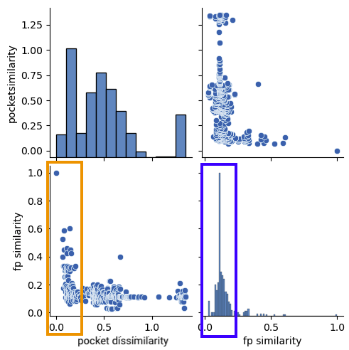
In the orange box on Figure 2 several ligands with some similarity to DZ8 are identified in very similar binding sites (pocket dissimilarity close to 0). More dissimilar binding sites do not seem to bind this class of ligands. This points into the direction that this series of compounds binds clearly to a particular conformation (or induces it, or both). It is also interesting to note that the majority of other compounds in the set are significantly dissimilar to the query ligand.

Figure 3: Distribution of ligand similarity vs pocket similarity values when using 6b9a ligand PA7 as reference

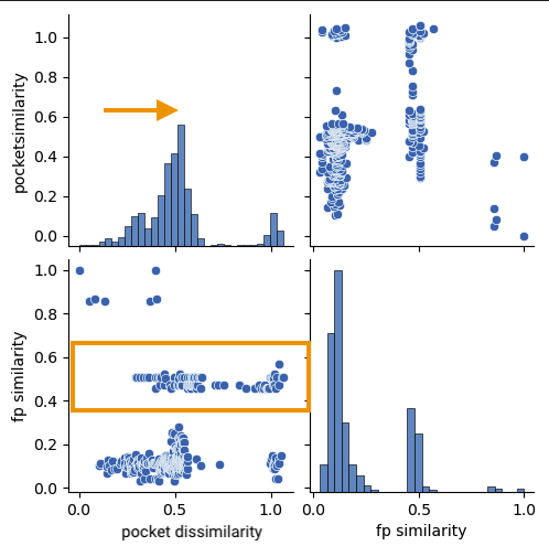
On figure Figure 3 we can see a very different distribution. Here we have an ATP analog as query ligand & the corresponding binding site. It is very interesting to observe the skewness to more dissimilar binding sites compared to 6b9a. Despite the dissimilarity on binding sites we can see a large cluster of ligands with around 0.5 Tanimoto similarity to PA7. This cluster encompasses ATP & all the closer analogs. This example is a very good one to illustrate the complexity behind the theory of similar ligands bind to similar binding sites. ATP analogs clearly accomodate for a larger variety of binding site conformations & mutations than the compound series around DZ8 does. We could then even imagine that DZ8 is conformation selective & has a few hallmarks of a more specific inhibitor. That’s a bit far fetched for a comparison with a plain ATP analog here, but it appears to go into that direction nevertheless.

References

Eguida, Merveille, and Didier Rognan. 2022. “Estimating the Similarity Between Protein Pockets.” International Journal of Molecular Sciences 23 (20): 12462. https://doi.org/10.3390/ijms232012462.

Kellenberger, Esther, Claire Schalon, and Didier Rognan. 2008. “How to Measure the Similarity Between Protein Ligand-Binding Sites?” Current Computer Aided-Drug Design 4 (3): 209–20. https://doi.org/10.2174/157340908785747401.

Kunzmann, Patrick, and Kay Hamacher. 2018. “Biotite: A Unifying Open Source Computational Biology Framework in Python.” BMC Bioinformatics 19 (1). https://doi.org/10.1186/s12859-018-2367-z.

Sreeramulu, Sridhar, Hendrik R. A. Jonker, Thomas Langer, Christian Richter, C. Roy D. Lancaster, and Harald Schwalbe. 2009. “The Human Cdc37\(\cdotp\)Hsp90 Complex Studied by Heteronuclear NMR Spectroscopy.” Journal of Biological Chemistry 284 (6): 3885–96. https://doi.org/10.1074/jbc.m806715200.