Binding Site Comparison Benchmarks - I - Binding sites on the same protein

Summary

In this article I’ll go through the overall thought process of setting up a benchmark set for the same binding site on the same protein. For the sake of simplicity I’ll do it for a single target to evaluate the performance of a binding site comparison algorithm. I’ll try to provide code whenever possible against public resources or snippets if a bit of scripting is needed. I will for sure run into dead ends (I won’t describe all of these 😬) and as a result I’ll have to make some decisions & put other things aside. In order to keep track of things I put aside I’ll use a side-note throughout the post to track all of these & make a summary of how to address or amend them later.

Things to keep in mind

• listing goes here

The target binding site

In order to show the overall process, let’s start with a well studied & relatively easy target, HSP90. A usual guinea pig since my PhD in Xavier Barril’s lab, but it’s a good example to show without exploring too much in super large protein families in the beginning. The aim of this post is to derive several approaches on how to set up a proper dataset and later apply that to other targets.

HSP90

The heat shock protein 90 is a rather abundant protein in the cell and helps during protein folding of not yet formed proteins, or protects already folded proteins from external stress (thermal stress for instance) - thus HSP = Heat Shock Protein. Let’s start with HSP90 alpha from the homo sapiens. Several kinases are dependent (activated) on HSP90, especially those acting as hub (Citri et al. (2006)). This is one of the reasons why HSP90 has been investigated as potential drug target for treatment of several forms of cancer. The action of HSP is dependent on ATP and the dephosphorylation of this molecule & the ATP binding site is located on a particular part of the N-terminal domain of HSP90. This will be the binding site to focus on here.

Why HSP90 as a first example

• HSP90 has a lot of structures available in the public domain
• It’s not part of any gigantic protein family (kinases, GPCR’s etc), which keeps the initial comparison space to cover a bit smaller and easier to manage
• The fold of the protein is still conserved among several other proteins, so there’s matter for detecting expected similarities
• It binds ATP, such as a lot of proteins in nature - which is interesting for the if I bind the same molecule I must be similar conundrum
• The binding site can undergo important conformational changes, which is good to evaluate sensity on conformation
• Water plays a very important role upon binding of small molecules into the ATP binding site

Domain architecture

HSP90 alpha human is composed of two domains: - the N-terminal Histidine kinase, DNA gyrase B and HSP90-like ATPase domain (ranging from amino acid 40 to 193) - the C-terminal HSP90 protein domain (196-714)

The ATP binding site of interest is on the N-terminal part and this is the part that you have the most crystal structures in the RCSB today. A full length Alphafold model is also available in the public domain, but I won’t discuss any of that here for now. NB: there appears to be another ATP binding site on the C-terminal part, that is only accessible when activated - so interesting to maybe look out for that one as well (Soti et al. (2003)). But again, not the main purpose of this post.

The topology of the ATP binding site (N-ter)

Code

// Create drawing area
divNGL = html`<div style="width:800px;height:600px;position:relative"></div>`;

Figure 1: Overview of N-terminal domain of human HSP90, canonical isoform

Code

NGL = require("ngl@next");
// Create trajectory object
stage = new NGL.Stage(divNGL, { backgroundColor: "black",cameraType: "orthographic"});
pdbString = await FileAttachment("3t0z.pdb").blob();
structure = await stage.loadFile(pdbString, {ext: "pdb", asTrajectory: false})
structure.addRepresentation("cartoon",{ "sele": "protein", "color": "residueindex"});

Code

structure.addRepresentation("ball+stick",{ "sele": "hetero and _C", "color": "yellow"});

Code

structure.addRepresentation("ball+stick",{ "sele": "hetero", "color": "element"});

Code

structure.addRepresentation("licorice",{ "sele": "47-55 or 91 or 93 or 96-97 or 98 or 102 or 106 or 107 or 112 or 132-139 or 150 or 162 or or 186", "color": "element"});

Code

structure.addRepresentation("contact",{ "sele": "47-55 or 91 or 93 or 96-97 or 98 or 102 or 106 or 107 or 112 or 132-139 or 150 or 162 or or 186 or ligand or water", "color": "element"});

Code

structure.autoView();

The binding site is composed of a section containing the adenin moiety which is characterized by a beta sheet at the bottom of the site, and two helices lining the site. The sidechains exposed to the binding site lumen are globally hydrophobic, a part from the very important aspartate 93, which is interacting directly with the adenine moiety. The adenine moiety is surrounded by water molecules and several of these waters are important hallmarks of several HSP90 binders. The ribose moiety is not forming any H-bonds with the protein itself but has hydroxyls oriented towards the solvent. The ether of the ribose is oriented towards the valine 107, adjacent to a rather hydrophobic part of the pocket coated by Y139, F138 and W162. The triphospate is solvent exposed and interacting with a small helix-loop-helix motive which, as we will probably see a bit later part of the more mobile regions of the binding site.

Establishing a reference set

Now we have defined a binding site of interest, let’s try to establish first a few obvious scenarios one might want to cover with a pocket comparison method. In my previous post I stated that the principle use case for binding site comparison methods that I’m focusing on is large scale comparison or screening for drug discovery purposes. The underlying use cases that I’m mainly interested in are NOT protein function prediction, but rather the prediction of potential counter targets, or extracting bound ligands from related binding sites to inform structurally during my compound design cycle. The subsequent steps I’ll outline in this post depend very much on the use I want to make of binding site comparison methods. As a result, what I’ll discuss here might very well not apply to other use cases of binding site comparison methods.

Let’s consider that we are working on a drug design project on the HSP90 N-terminal ATP binding site and we have our favourite structure of HSP90 as starting point, i.e. 4cwr.

If I want to find similar binding sites to my query binding site vs all known/putative binding sites, what hits I’d expect to get first in the hitlist when screening large structure databases like the RCSB PDB or Alphafold?:

1. the ATP binding site of other HSP90 alpha human structures with the same overall conformation (more or less) - same sequence & conformation
2. the ATP binding site of other HSP90 human isoforms with a similar conformation - likely locally identical sequences & conformation
3. the ATP binding site of HSP90 sequences from other species with a similar conformation - locally very similar sequences
4. all of the above but with a bit different conformations - conformations
5. the ATP binding site of close homologs (sequence - families etc) to the query structure - similar sequences
6. the ATP binding sites of proteins sharing the same fold as HSP90 - same fold
7. nucleotide binding sites with similar interaction patterns but dissimar fold - same interactions
8. all binding sites binding ATP must be similar (that’s provocative on purpose …) - same ligand
9. unexpected & unrelated / unknown similarities - nightmare

I’d expect to retrieve hits also most likely (not guaranteed) in that particular order as well. These first five give a graduation up to which level another ATP binding site could be potentially close to the HSP90 binding site. These are the obvious clusters of sequences, structures & conformations one would expect to find. As a result, one can use this type of graduation also for validating binding site comparison methods. One major difference with the setting I’m laying out here, is that the background data encompasses the full RCSB PDB structures containing all ligand binding sites + putative binding sites (empty clefts). This sets the approach I’m suggesting into stark contrast with previous benchmark sets. Such previous sets were classically composed of a list of expected matches of binding site pairs and decoys (expected mismatches). As Vincent Le Guilloux states it fairly regularly, if you can avoid a threshold effect, avoid it! This is exactly such a case where a discrete split between a match & a mismatch is typically introduced. As a result my background data (what one usually calls a decoy) would be the full pocketome. As a result I’ll try to use metrics of success that measure, how many of the potentially expected hits are found before a bulk of less expected hits & why.

In this post I’ll go through the steps to create the dataset corresponding the very first & the easiest steps. I’ll cover 2 to 5 in different posts, as already this one here is getting fairly long & complex. The situation 7 & 8 are a bit more tricky to set up. As for 9 - that’s the big issue with binding site comparison benchmarking - you don’t know until you know, but I’ll try to do a bit of my homework on that as well!

Same sequence & conformation

Alright, here we go … the same sequence is the easiest case of all of them & several previous studies included a selection of structures, but as you’ll see even here to do things properly it gets quickly tricky. The following script will cover the required steps:

• define the sets of residues of our reference binding site
• gather all structures (PDB codes) containing a resolved HSP90 alpha human N terminal domain
• filter out structures with mutations on binding site residues compared to the wild type
• get an all by all comparison of the binding sites (structurally speaking) which would allow for some rough clustering of conformations

Defining the binding site

On Figure 1 we already displayed a set of amino-acids on the HSP90 structure surrounding the binding site. Let’s get a list defined by hand getting all residues:

Table 1: ATP binding site residue selection on structure 4cwr

WT Sequence Position	Chain	Residue
E47	A	E47
L48	A	L48
N51	A	N51
S52	A	S52
D54	A	D54
A55	A	A55
K58	A	K58
D93	A	D93
G95	A	G95
I96	A	I96
G97	A	G97
M98	A	M98
N106	A	N106
L107	A	L107
K112	A	K112
I131	A	I131
G132	A	G132
Q133	A	Q133
F134	A	F134
G135	A	G135
V136	A	V136
G137	A	G137
F138	A	F138
Y139	A	Y139
T152	A	Y152
G183	A	G183
T184	A	T184
V186	A	V186

Gathering all PDB codes containing the site

Now we have the protein & binding site of interest defined, we can gather all RCSB PDB structures containing that portion without mutations compared to the WT sequence. The uniprot accession for the human HSP90 is P07900 (HS90A_HUMAN) & we will use the WT HSP90 alpha here as reference. NB: there is a known splice variant adding another 123 amino acids in front of ther canonical N-terminal part of the protein.

In order to retrieve all PDB structures of a particular protein sequences one can use various resources. The obvious one to start with would be uniprot, ncbi or the RCSB itself.

From uniprot we can use something like the ID mapping service for instance:

Code

# Code adapted from here: https://www.uniprot.org/help/id_mapping
import re
import time
import json
import zlib
from urllib.parse import urlparse, parse_qs, urlencode
import requests
from requests.adapters import HTTPAdapter, Retry


POLLING_INTERVAL = 3
API_URL = "https://rest.uniprot.org"


retries = Retry(total=5, backoff_factor=0.25, status_forcelist=[500, 502, 503, 504])
session = requests.Session()
session.mount("https://", HTTPAdapter(max_retries=retries))


def check_response(response):
    try:
        response.raise_for_status()
    except requests.HTTPError:
        print(response.json())
        raise


def submit_id_mapping(from_db, to_db, ids):
    request = requests.post(
        f"{API_URL}/idmapping/run",
        data={"from": from_db, "to": to_db, "ids": ",".join(ids)},
    )
    check_response(request)
    return request.json()["jobId"]


def get_next_link(headers):
    re_next_link = re.compile(r'<(.+)>; rel="next"')
    if "Link" in headers:
        match = re_next_link.match(headers["Link"])
        if match:
            return match.group(1)


def check_id_mapping_results_ready(job_id):
    while True:
        request = session.get(f"{API_URL}/idmapping/status/{job_id}")
        check_response(request)
        j = request.json()
        if "jobStatus" in j:
            if j["jobStatus"] == "RUNNING":
                print(f"Retrying in {POLLING_INTERVAL}s")
                time.sleep(POLLING_INTERVAL)
            else:
                raise Exception(j["jobStatus"])
        else:
            return bool(j["results"] or j["failedIds"])


def get_batch(batch_response, file_format, compressed):
    batch_url = get_next_link(batch_response.headers)
    while batch_url:
        batch_response = session.get(batch_url)
        batch_response.raise_for_status()
        yield decode_results(batch_response, file_format, compressed)
        batch_url = get_next_link(batch_response.headers)


def combine_batches(all_results, batch_results, file_format):
    if file_format == "json":
        for key in ("results", "failedIds"):
            if key in batch_results and batch_results[key]:
                all_results[key] += batch_results[key]
    elif file_format == "tsv":
        return all_results + batch_results[1:]
    else:
        return all_results + batch_results
    return all_results


def get_id_mapping_results_link(job_id):
    url = f"{API_URL}/idmapping/details/{job_id}"
    request = session.get(url)
    check_response(request)
    return request.json()["redirectURL"]


def decode_results(response, file_format, compressed):
    if compressed:
        decompressed = zlib.decompress(response.content, 16 + zlib.MAX_WBITS)
        if file_format == "json":
            j = json.loads(decompressed.decode("utf-8"))
            return j
        elif file_format == "tsv":
            return [line for line in decompressed.decode("utf-8").split("\n") if line]
        elif file_format == "xlsx":
            return [decompressed]
        else:
            return decompressed.decode("utf-8")
    elif file_format == "json":
        return response.json()
    elif file_format == "tsv":
        return [line for line in response.text.split("\n") if line]
    elif file_format == "xlsx":
        return [response.content]
    return response.text



def print_progress_batches(batch_index, size, total):
    n_fetched = min((batch_index + 1) * size, total)
    print(f"Fetched: {n_fetched} / {total}")


def get_id_mapping_results_search(url):
    parsed = urlparse(url)
    query = parse_qs(parsed.query)
    file_format = query["format"][0] if "format" in query else "tsv"
    if "size" in query:
        size = int(query["size"][0])
    else:
        size = 500
        query["size"] = size
    compressed = (
        query["compressed"][0].lower() == "true" if "compressed" in query else False
    )
    parsed = parsed._replace(query=urlencode(query, doseq=True))
    url = parsed.geturl()
    request = session.get(url)
    check_response(request)
    results = decode_results(request, file_format, compressed)
    total = int(request.headers["x-total-results"])
    print_progress_batches(0, size, total)
    for i, batch in enumerate(get_batch(request, file_format, compressed), 1):
        results = combine_batches(results, batch, file_format)
        print_progress_batches(i, size, total)
    return results

job_id = submit_id_mapping(
    from_db="UniProtKB_AC-ID", to_db="PDB", ids=["P07900"]
)
if check_id_mapping_results_ready(job_id):
    link = get_id_mapping_results_link(job_id)
    results = get_id_mapping_results_search(link)
    results_python = json.loads(results[0])["results"]
    # print(results_python)
    up_pdbcodes=[element["to"].lower() for element in results_python]
    print(up_pdbcodes)

Fetched: 328 / 328
['1byq', '1osf', '1uy6', '1uy7', '1uy8', '1uy9', '1uyc', '1uyd', '1uye', '1uyf', '1uyg', '1uyh', '1uyi', '1uyk', '1uyl', '1yc1', '1yc3', '1yc4', '1yer', '1yes', '1yet', '2bsm', '2bt0', '2bug', '2byh', '2byi', '2bz5', '2c2l', '2ccs', '2cct', '2ccu', '2fwy', '2fwz', '2h55', '2jjc', '2k5b', '2qf6', '2qfo', '2qg0', '2qg2', '2uwd', '2vci', '2vcj', '2wi1', '2wi2', '2wi3', '2wi4', '2wi5', '2wi6', '2wi7', '2xab', '2xdk', '2xdl', '2xds', '2xdu', '2xdx', '2xhr', '2xht', '2xhx', '2xjg', '2xjj', '2xjx', '2xk2', '2ye2', '2ye3', '2ye4', '2ye5', '2ye6', '2ye7', '2ye8', '2ye9', '2yea', '2yeb', '2yec', '2yed', '2yee', '2yef', '2yeg', '2yeh', '2yei', '2yej', '2yi0', '2yi5', '2yi6', '2yi7', '2yjw', '2yjx', '2yk2', '2yk9', '2ykb', '2ykc', '2yke', '2yki', '2ykj', '3b24', '3b25', '3b26', '3b27', '3b28', '3bm9', '3bmy', '3d0b', '3eko', '3ekr', '3ft5', '3ft8', '3hek', '3hhu', '3hyy', '3hyz', '3hz1', '3hz5', '3inw', '3inx', '3k97', '3k98', '3k99', '3mnr', '3o0i', '3ow6', '3owb', '3owd', '3q6m', '3q6n', '3qdd', '3qtf', '3r4m', '3r4n', '3r4o', '3r4p', '3r91', '3r92', '3rkz', '3rlp', '3rlq', '3rlr', '3t0h', '3t0z', '3t10', '3t1k', '3t2s', '3tuh', '3vha', '3vhc', '3vhd', '3wha', '3wq9', '4aif', '4awo', '4awp', '4awq', '4b7p', '4bqg', '4bqj', '4cgq', '4cgu', '4cgv', '4cgw', '4cwf', '4cwn', '4cwo', '4cwp', '4cwq', '4cwr', '4cws', '4cwt', '4eeh', '4eft', '4efu', '4egh', '4egi', '4egk', '4fcp', '4fcq', '4fcr', '4hy6', '4jql', '4l8z', '4l90', '4l91', '4l93', '4l94', '4lwe', '4lwf', '4lwg', '4lwh', '4lwi', '4nh7', '4nh8', '4o04', '4o05', '4o07', '4o09', '4o0b', '4r3m', '4u93', '4w7t', '4xip', '4xiq', '4xir', '4xit', '4ykq', '4ykr', '4ykt', '4yku', '4ykw', '4ykx', '4yky', '4ykz', '5cf0', '5fnc', '5fnd', '5fnf', '5ggz', '5j20', '5j27', '5j2v', '5j2x', '5j64', '5j6l', '5j6m', '5j6n', '5j80', '5j82', '5j86', '5j8m', '5j8u', '5j9x', '5lny', '5lnz', '5lo0', '5lo1', '5lo5', '5lo6', '5lq9', '5lr1', '5lr7', '5lrl', '5lrz', '5ls1', '5m4e', '5m4h', '5nyh', '5nyi', '5oci', '5od7', '5odx', '5t21', '5vyy', '5xqd', '5xqe', '5xr5', '5xr9', '5xrb', '5xrd', '5xre', '5zr3', '6b99', '6b9a', '6ceo', '6cyg', '6cyh', '6ei5', '6el5', '6eln', '6elo', '6elp', '6ey8', '6ey9', '6eya', '6eyb', '6f1n', '6fcj', '6fdp', '6gp4', '6gp8', '6gpf', '6gph', '6gpo', '6gpp', '6gpr', '6gpt', '6gpw', '6gpy', '6gq6', '6gqr', '6gqs', '6gqu', '6gr1', '6gr3', '6gr4', '6gr5', '6hhr', '6ksq', '6lr9', '6lsz', '6lt8', '6lti', '6ltk', '6n8x', '6olx', '6tn4', '6tn5', '6u98', '6u99', '6u9a', '6u9b', '7dmc', '7krj', '7kw7', '7l7i', '7l7j', '7lsz', '7lt0', '7ry1', '7s8y', '7s8z', '7s90', '7s95', '7s98', '7s99', '7s9f', '7s9g', '7s9h', '7s9i', '8agi', '8agj', '8agl']

This results in a list of 328 structures. As uniprot isn’t the only source to get that info, let’s check what comes out of the same type of query against the RCSB PDB, should be the same, right?

Code

inputjson="""{
  "query": {
    "type": "group",
    "nodes": [
      {
        "type": "terminal",
        "service": "text",
        "parameters": {
          "attribute": "rcsb_polymer_entity_container_identifiers.reference_sequence_identifiers.database_accession",
          "operator": "in",
          "value": [
            "P07900"
          ]
        }
      },
      {
        "type": "terminal",
        "service": "text",
        "parameters": {
          "attribute": "rcsb_polymer_entity_container_identifiers.reference_sequence_identifiers.database_name",
          "operator": "exact_match",
          "value": "UniProt",
          "negation": false
        }
      }
    ],
    "logical_operator": "and",
    "label": "nested-attribute"
  },
  "return_type": "entry",
  "request_options": {
    "paginate": {
      "start": 0,
      "rows": 500
    },
    "results_content_type": [
      "experimental"
    ],
    "sort": [
      {
        "sort_by": "score",
        "direction": "desc"
      }
    ],
    "scoring_strategy": "combined"
  }
}"""
url="https://search.rcsb.org/rcsbsearch/v2/query?json="+inputjson
response=requests.get(url)
tmp=json.loads(response.text)["result_set"]
rcsb_pdbcodes=[element["identifier"].lower() for element in tmp]
print(len(rcsb_pdbcodes))
print(rcsb_pdbcodes)

331
['1byq', '1osf', '1uy6', '1uy7', '1uy8', '1uy9', '1uyc', '1uyd', '1uye', '1uyf', '1uyg', '1uyh', '1uyi', '1uyk', '1uyl', '1yc1', '1yc3', '1yc4', '1yer', '1yes', '1yet', '2bsm', '2bt0', '2bug', '2byh', '2byi', '2bz5', '2c2l', '2ccs', '2cct', '2ccu', '2fwy', '2fwz', '2h55', '2jjc', '2k5b', '2qf6', '2qfo', '2qg0', '2qg2', '2uwd', '2vci', '2vcj', '2wi1', '2wi2', '2wi3', '2wi4', '2wi5', '2wi6', '2wi7', '2xab', '2xdk', '2xdl', '2xds', '2xdu', '2xdx', '2xhr', '2xht', '2xhx', '2xjg', '2xjj', '2xjx', '2xk2', '2ye2', '2ye3', '2ye4', '2ye5', '2ye6', '2ye7', '2ye8', '2ye9', '2yea', '2yeb', '2yec', '2yed', '2yee', '2yef', '2yeg', '2yeh', '2yei', '2yej', '2yi0', '2yi5', '2yi6', '2yi7', '2yjw', '2yjx', '2yk2', '2yk9', '2ykb', '2ykc', '2yke', '2yki', '2ykj', '3b24', '3b25', '3b26', '3b27', '3b28', '3bm9', '3bmy', '3d0b', '3eko', '3ekr', '3ft5', '3ft8', '3hek', '3hhu', '3hyy', '3hyz', '3hz1', '3hz5', '3inw', '3inx', '3k97', '3k98', '3k99', '3mnr', '3o0i', '3ow6', '3owb', '3owd', '3q6m', '3q6n', '3qdd', '3qtf', '3r4m', '3r4n', '3r4o', '3r4p', '3r91', '3r92', '3rkz', '3rlp', '3rlq', '3rlr', '3t0h', '3t0z', '3t10', '3t1k', '3t2s', '3tuh', '3vha', '3vhc', '3vhd', '3wha', '3wq9', '4aif', '4awo', '4awp', '4awq', '4b7p', '4bqg', '4bqj', '4cgq', '4cgu', '4cgv', '4cgw', '4cwf', '4cwn', '4cwo', '4cwp', '4cwq', '4cwr', '4cws', '4cwt', '4eeh', '4eft', '4efu', '4egh', '4egi', '4egk', '4fcp', '4fcq', '4fcr', '4hy6', '4jql', '4l8z', '4l90', '4l91', '4l93', '4l94', '4lwe', '4lwf', '4lwg', '4lwh', '4lwi', '4nh7', '4nh8', '4o04', '4o05', '4o07', '4o09', '4o0b', '4r3m', '4u93', '4w7t', '4xip', '4xiq', '4xir', '4xit', '4ykq', '4ykr', '4ykt', '4yku', '4ykw', '4ykx', '4yky', '4ykz', '5cf0', '5fnc', '5fnd', '5fnf', '5ggz', '5j20', '5j27', '5j2v', '5j2x', '5j64', '5j6l', '5j6m', '5j6n', '5j80', '5j82', '5j86', '5j8m', '5j8u', '5j9x', '5lny', '5lnz', '5lo0', '5lo1', '5lo5', '5lo6', '5lq9', '5lr1', '5lr7', '5lrl', '5lrz', '5ls1', '5m4e', '5m4h', '5nyh', '5nyi', '5oci', '5od7', '5odx', '5t21', '5vyy', '5xqd', '5xqe', '5xr5', '5xr9', '5xrb', '5xrd', '5xre', '5zr3', '6b99', '6b9a', '6ceo', '6cyg', '6cyh', '6ei5', '6el5', '6eln', '6elo', '6elp', '6ey8', '6ey9', '6eya', '6eyb', '6f1n', '6fcj', '6fdp', '6gp4', '6gp8', '6gpf', '6gph', '6gpo', '6gpp', '6gpr', '6gpt', '6gpw', '6gpy', '6gq6', '6gqr', '6gqs', '6gqu', '6gr1', '6gr3', '6gr4', '6gr5', '6hhr', '6ksq', '6lr9', '6lsz', '6lt8', '6lti', '6ltk', '6n8x', '6olx', '6tn4', '6tn5', '6u98', '6u99', '6u9a', '6u9b', '7dmc', '7krj', '7kw7', '7l7i', '7l7j', '7lsz', '7lt0', '7rxz', '7ry0', '7ry1', '7s8y', '7s8z', '7s90', '7s95', '7s98', '7s99', '7s9f', '7s9g', '7s9h', '7s9i', '7ur3', '8agi', '8agj', '8agl']

From the RCSB we get 3 more structures than from Uniprot. Let’s see what the difference between both lists of pdb codes is:

['7rxz', '7ry0', '7ur3']

Again a bit worrisome difference between the RCSB & Uniprot. An NCBI search seems to give yet another number of 273 structures. NB: when you have a look at the P07900 sequence cluster page of the RCSB, one gets 332 hits instead, so even one more than through the API. The RCSB seems to handle the uniprot accession code a bit differently from the Polymer Entity Group ID (or there’s an issue with the data of one structure) when searching through the advanced search through the UI. I’ll have to check with the RCSB folks on that one. For now I’ll stick to the 331 structures from the previous API call vs the RCSB.

Things to keep in mind

• Uniprot accession vs polymer entity group ID handling to be clarified with RCSB folks

As we can see in Table 1 the residues encompassing our binding site of interest range from amino acid E47 on the WT sequence to V186. So now we need to know whether the region expressed & resolved in each crystal structure includes our binding site of interest. This can now be done with a graphQL query versus the RCSB (after a lot of trial & error 😒 ). NB: I directly filter out structures (18) that contain mutations versus wild type.

Code

query="""
{
  entries(entry_ids: """+str(rcsb_pdbcodes).replace("'","\"")+""")
  {
    rcsb_id
    
    polymer_entities {
      rcsb_polymer_entity_container_identifiers {
        entity_id
        asym_ids
        auth_asym_ids
        reference_sequence_identifiers {
          database_name
          database_accession
        }
      }
      rcsb_polymer_entity_align{
        
  reference_database_name
        aligned_regions{
          entity_beg_seq_id
          length
          ref_beg_seq_id
        }
        
      }
      entity_poly {
        pdbx_seq_one_letter_code_can
        rcsb_sample_sequence_length
        type
        rcsb_mutation_count
      }
      rcsb_polymer_entity {
        formula_weight
      }
    }
  }
}
"""

# ugly I know, but does the job here
def extractSequenceRegions(data):
  result={}
  
  for entry in data:  
    result[entry["rcsb_id"]]=[]
    for entity in entry["polymer_entities"]:
      # print(entity["rcsb_polymer_entity_container_identifiers"])
      if entity["entity_poly"]["rcsb_mutation_count"]==0:
        for idx,identifier in enumerate(entity["rcsb_polymer_entity_container_identifiers"]["reference_sequence_identifiers"]):
          if identifier["database_name"]=="UniProt" and identifier["database_accession"]=="P07900":
            if entity["rcsb_polymer_entity_align"][idx]["reference_database_name"]=="UniProt":
              for region in entity["rcsb_polymer_entity_align"][idx]["aligned_regions"]:
                result[entry["rcsb_id"]].append((region["ref_beg_seq_id"],region["ref_beg_seq_id"]+region["length"]))
  return result

residuelist=[47,48,51,52,54,55,58,93,95,96,97,98,106,107,112,131,132,133,134,135,136,137,138,139,152,183,184,186]

url=f"https://data.rcsb.org/graphql?query={query}"
response=requests.get(url)
dataRCSBGQL=response.json()["data"]["entries"]


resolved_regions=extractSequenceRegions(dataRCSBGQL)

selectedPdbCodes=[]
for pdbCode in resolved_regions:
  for mapping in resolved_regions[pdbCode]:
    if(all(i>=mapping[0] and i<=mapping[1] for i in residuelist)):
      selectedPdbCodes.append(pdbCode)

print(selectedPdbCodes)
print(str(len(selectedPdbCodes)) + " structures identified")

['1BYQ', '1OSF', '1UY6', '1UY7', '1UY8', '1UY9', '1UYC', '1UYD', '1UYE', '1UYF', '1UYG', '1UYH', '1UYI', '1UYK', '1UYL', '1YC1', '1YC3', '1YC4', '1YER', '1YES', '1YET', '2BSM', '2BT0', '2BYH', '2BYI', '2BZ5', '2CCS', '2CCT', '2CCU', '2FWY', '2FWZ', '2H55', '2JJC', '2K5B', '2QF6', '2QFO', '2QG0', '2QG2', '2UWD', '2VCI', '2VCJ', '2WI1', '2WI2', '2WI3', '2WI4', '2WI5', '2WI6', '2WI7', '2XAB', '2XDK', '2XDL', '2XDS', '2XDU', '2XDX', '2XHR', '2XHT', '2XHX', '2XJG', '2XJJ', '2XJX', '2XK2', '2YE2', '2YE3', '2YE4', '2YE5', '2YE6', '2YE7', '2YE8', '2YE9', '2YEA', '2YEB', '2YEC', '2YED', '2YEE', '2YEF', '2YEG', '2YEH', '2YEI', '2YEJ', '2YI0', '2YI5', '2YI6', '2YI7', '2YJW', '2YJX', '2YK2', '2YK9', '2YKB', '2YKC', '2YKE', '2YKI', '2YKJ', '3B24', '3B25', '3B26', '3B27', '3B28', '3BM9', '3BMY', '3D0B', '3EKO', '3EKR', '3FT5', '3FT8', '3HEK', '3HHU', '3HYY', '3HYZ', '3HZ1', '3HZ5', '3INW', '3INX', '3K97', '3K98', '3K99', '3MNR', '3O0I', '3OW6', '3OWB', '3OWD', '3QDD', '3QTF', '3R4M', '3R4N', '3R4O', '3R4P', '3R91', '3R92', '3RKZ', '3RLP', '3RLQ', '3RLR', '3T0H', '3T0Z', '3T10', '3T1K', '3T2S', '3TUH', '3VHA', '3VHC', '3VHD', '3WHA', '3WQ9', '4AWO', '4AWP', '4AWQ', '4B7P', '4BQG', '4BQJ', '4CWF', '4CWN', '4CWO', '4CWP', '4CWQ', '4CWR', '4CWS', '4CWT', '4EEH', '4EFT', '4EFU', '4EGH', '4EGI', '4EGK', '4FCP', '4FCQ', '4FCR', '4HY6', '4JQL', '4L8Z', '4L90', '4L91', '4L93', '4L94', '4LWE', '4LWF', '4LWG', '4LWH', '4LWI', '4NH7', '4NH8', '4O04', '4O05', '4O07', '4O09', '4O0B', '4R3M', '4U93', '4W7T', '4XIP', '4XIQ', '4XIR', '4XIT', '4YKQ', '4YKR', '4YKT', '4YKU', '4YKW', '4YKX', '4YKY', '4YKZ', '5CF0', '5FNC', '5FND', '5FNF', '5GGZ', '5J20', '5J27', '5J2V', '5J2X', '5J64', '5J6L', '5J6M', '5J6N', '5J82', '5J86', '5J8M', '5J8U', '5J9X', '5LNY', '5LNZ', '5LO0', '5LO1', '5LO5', '5LO6', '5LQ9', '5LR1', '5LR7', '5LRL', '5LRZ', '5LS1', '5M4E', '5M4H', '5NYH', '5NYI', '5OCI', '5OD7', '5ODX', '5T21', '5VYY', '5XQD', '5XQE', '5XR5', '5XR9', '5XRB', '5XRD', '5XRE', '5ZR3', '6B99', '6B9A', '6CEO', '6CYG', '6CYH', '6EI5', '6EL5', '6ELN', '6ELO', '6ELP', '6EY8', '6EY9', '6EYA', '6EYB', '6F1N', '6FCJ', '6GPR', '6GPT', '6GPW', '6GPY', '6GQ6', '6GQR', '6HHR', '6LR9', '6LSZ', '6LT8', '6LTI', '6LTK', '6N8X', '6TN4', '6TN5', '6U99', '6U9B', '7DMC', '7KRJ', '7KW7', '7L7I', '7L7J', '7LSZ', '7LT0', '7S8Y', '7S8Z', '7S90', '7S95', '7S98', '7S99', '7S9F', '7S9G', '7S9H', '7S9I', '7UR3', '8AGI']
299 structures identified

Now we have our list of 299 WT structures with the ATP binding site resolved. NB: you might have noticed that I’m not taking the resolution, Rfree or Rwork into account for the structure selection here. That’s on purpose. During the subsequent clustering step I’ll still check if all residues of interest of the binding site are resolved (or have been modelled by the crystallographer).

Things to keep in mind

• Uniprot accession vs polymer entity group ID handling to be clarified with RCSB folks
• Don’t forget to check if all sidechains of the binding site are resolved in the selected structures

Cluster by conformation

The ATP binding site of HSP90 can be fairly flexible in specific regions. In order to evaluate a pocket comparison method’s sensitivity to sidechain or backbone movements we can split down the 299 structures we just identified to smaller clusters of very similar conformations. This will allow us later to run tests using different pocket comparison algorithms.

Already doing all the previous work was not as straightforward as what one might have expected, but it’s still doable. Especially with the API available now from the RCSB. A few years back one had to rely on predictions from the SIFTS project from Dana et al. (2018) & Velankar et al. (2012).

Usually one relies then on superposing all structures onto a single reference frame & detect main differences, calculate RMSD’s etc. However, the structural superimpositioning poses the following challenges here:

1. in case of a multimer, shall we use all chains or all if the asymetric unit contains several copies of the same protein?
   • In theory we should assess if there are major differences between monomers or use the monomers as expected hit we should retrieve when comparing binding sites. Both should be covered by the overall dataset here so I’ll be lazy and will focus on the first chain
2. shall we use a standard Kabsch superimpositioning (Kabsch 1976) (local/global?) & overall root mean square deviation to assess the similarity between binding site conformations?
   • If I’m bringing this thing up, I think it’s important to address it properly. I’ll try to explain a bit in more detail why

Things to keep in mind

• Uniprot accession vs polymer entity group ID handling to be clarified with RCSB folks
• Don’t forget to check if all sidechains of the binding site are resolved in the selected structures
• Treat homo-multimers rationally in the data-set construction

Why isn’t standard superimpositioning enough?

I don’t have to write a ton of text here, citing the single, most relevant paper from Damm and Carlson (2006) should be argument enough 😁

But to showcase maybe a bit more clearly. HSP90 can adopt several conformations in different areas of the binding site:

Code

// Create drawing area
divNGL2 = html`<div style="width:800px;height:600px;position:relative"></div>`;

Figure 2: Comparison of distinct binding site conformations (3t0z,4cwr & 7l7j)

Code

stage2 = new NGL.Stage(divNGL2, { backgroundColor: "black",cameraType: "orthographic"});
pdbString1 = await FileAttachment("3t0z.pdb").blob();
structure1 = await stage2.loadFile(pdbString1, {ext: "pdb", asTrajectory: false})
structure1.addRepresentation("cartoon",{ "sele": "protein", "color": "#325E73"});

Code

structure1.addRepresentation("ball+stick",{ "sele": "ATP", "color": "element"});

Code

pdbString2 = await FileAttachment("pdbs/4cwr_aligned.pdb").blob();
structure2 = await stage2.loadFile(pdbString2, {ext: "pdb", asTrajectory: false})
structure2.addRepresentation("cartoon",{ "sele": "protein", "color": "#B69849"});

Code

pdbString3 = await FileAttachment("pdbs/7l7j_aligned.pdb").blob();
structure3 = await stage2.loadFile(pdbString3, {ext: "pdb", asTrajectory: false})
structure3.addRepresentation("cartoon",{ "sele": "protein", "color": "#B66049"});

Code

structure1.autoView("ATP");

So if you superimpose binding site residues only with a classical Kabsch algorithm you might alter significantly the positions of all binding site residues that appear to be stable (beta sheet & helix 44-58 for instance). Also clustering such superposed structures on differences on amino acid positions will yield sub-optimal results.

Furthermore, one should decouple the superimpositioning two structures from the similarity measurement of conformations once they are superimposed. With the classical Kabsch algorithm & the resulting RMSD, all of this is intertwined.

Kufareva and Abagyan (2011) already wrote about that topic and stated the properties of an ideal protein similarity measure as:

An ideal measure should allow both a single ‘summary’ number within a fixed range (e.g. 0% to 100%) and an underlying detailed vector or matrix representation. The single number must distinguish well between related (correct) and non-related (incorrect) structure pairs, i.e. its distributions on the two sets must overlap to a minimal possible degree. It has to be relevant, i.e. capture the nature of protein folding or protein interaction determinants rather than satisfy simple geometric criteria. It has to have the minimal number of parameters, which in turn need to be well justified and understandable. It has to be stable and robust against minor or fractional (affecting a small fraction of the model) experimental and modeling errors; such changes in the structures should not lead to major leaps in the calculated similarity measure values. It has to capture the similarities or differences between the structures at any given level of accuracy/resolution. Ideally, it should have an intuitive visual interpretation.

Kufareva and Abagyan (2011) however conclude that even distance weighted optimization & related cartesian space metrics are always prone to several issues. In the end they conclude that contact based metrics are more robust. So this is what I’ll be using here.

Contact based conformation comparison

At first I’m going to use some tools already existing in MDanalysis(Gowers et al. (2016),Michaud-Agrawal et al. (2011)), a popular python toolkit for MD trajectory analysis. It contains already prebuilt funtions to calculate the contact maps of a protein structure. But overall, you can achieve the same thing with any other toolkit & a lot of looping.

import MDAnalysis as mda
import numpy as np
from scipy.spatial.distance import cdist
from MDAnalysis.analysis import distances
import seaborn as sns
import gemmi
import matplotlib.pyplot as plt

filename="3t0z.pdb"
u = mda.Universe(filename)

residue_seqnums=[47,48,51,52,54,55,58,93,95,96,97,98,106,107,112,131,132,133,134,135,136,137,138,139,152,183,184,186]
residues = u.select_atoms('protein and name CA and resnum {}'.format(' '.join(map(str, residue_seqnums))))

distances3t0z = distances.distance_array(residues.positions, residues.positions)

sns.heatmap(distances3t0z,yticklabels=residue_seqnums,xticklabels=residue_seqnums,cmap="Blues",square=True)
plt.show()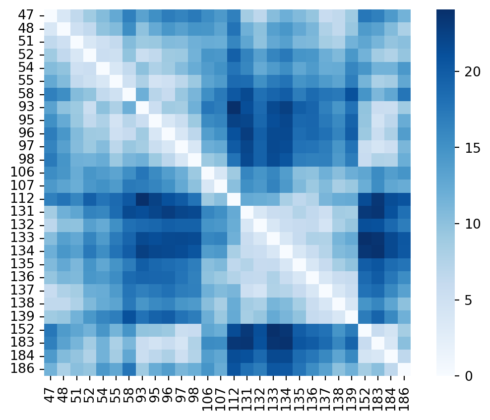

Figure 3: Contact matrix of alpha carbons of the ATP binding site of structure 3t0z

The code above has two main limitations that come to my mind. The first one is that the residue numbering I’m using is the canonical uniprot sequence one, but I’m not assured the residue numbering is the same in all HSP90 structures I selected. The second one is that I’m only computing distances between alpha carbons. This implies that I’ll only be able to measure differences in backbone conformations and as such important conformational changes. I won’t be able to detect subtle side-chain conformational changes. One could use an all atom distance matrix, or compute the center of mass for each residue & compare that instead. The time being let’s stick to alpha carbons. Also, I dont need to check for missing atoms in the structures for now with this simplification.

Things to keep in mind

• Uniprot accession vs polymer entity group ID handling to be clarified with RCSB folks
• Don’t forget to check if all sidechains of the binding site are resolved in the selected structures
• Treat homo-multimers rationally in the data-set construction
• Handle canonical residue numbering properly in distanceMatrix code
• Consider also optional side-chain sensitive distance calculations

Now let’s calculate the same distance matrix on another structure, for instance 4cwr.

Code

filename="pdbs/4cwr_aligned.pdb"
u = mda.Universe(filename)
residues = u.select_atoms('protein and name CA and resnum {}'.format(' '.join(map(str, residue_seqnums))))
distances4cwr = distances.distance_array(residues.positions, residues.positions)


fig, ax = plt.subplots(1,2)
sns.heatmap(distances3t0z,yticklabels=residue_seqnums,xticklabels=residue_seqnums,cmap="Blues",square=True,ax=ax[0])

sns.heatmap(distances4cwr,yticklabels=residue_seqnums,xticklabels=residue_seqnums,cmap="Blues",square=True,ax=ax[1])
plt.show()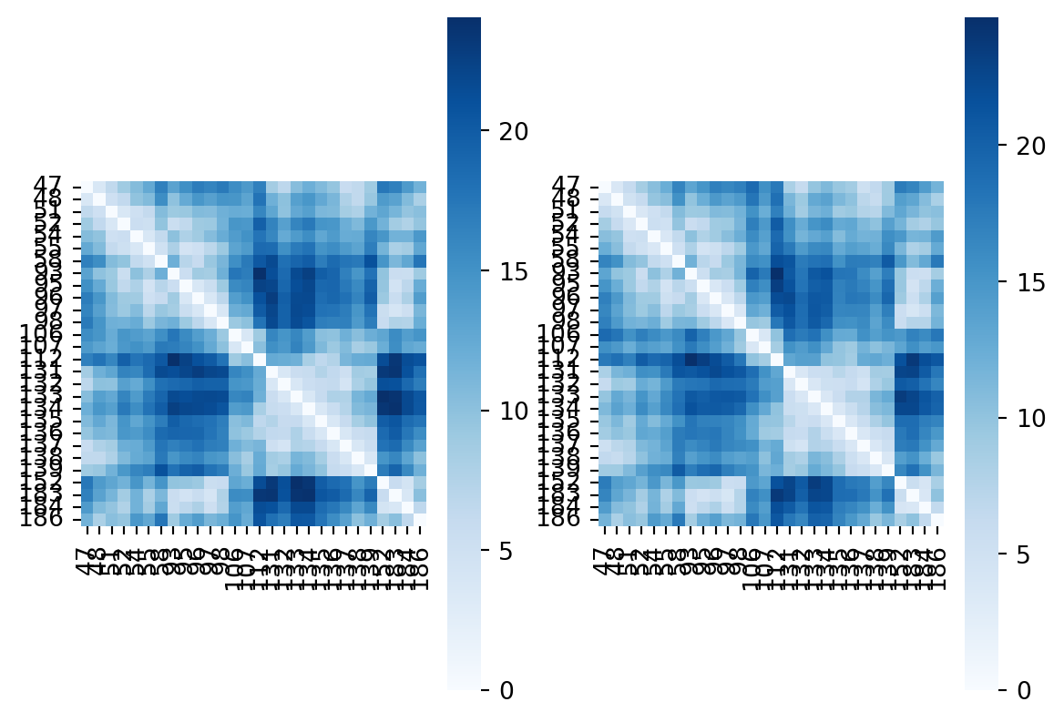

Figure 4: Comparison of distinct binding site conformations (3t0z,4cwr) using a CA contact matrix

Visual inspection won’t help a lot here. Let’s calculate the difference between the two matrices. I’ll call the resulting matrix a contact difference matrix from hereon. And check if we can spot the residues we observe to be moving significantly.

Code

distancematrix=np.abs(distances3t0z-distances4cwr)
sns.heatmap(distancematrix,yticklabels=residue_seqnums,xticklabels=residue_seqnums,cmap="Blues",square=True)
plt.show()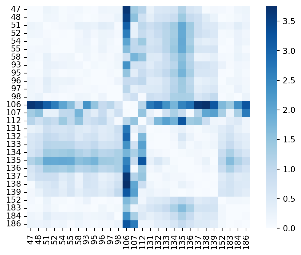

Figure 5: Comparison of distinct binding site conformations (3t0z,4cwr) using a contact difference matrix (colorscale in Angstroms)

That looks already a lot nicer. Here we can see that residues 106, 107 and 112 clearly move a lot when comparing both structures. Also the section 131-139 shows signficant motion when compared to residues 41-98. To understand better what is going on, let’s show both structures overlayed.

Code

// Create drawing area
divNGL3 = html`<div style="width:800px;height:600px;position:relative"></div>`;

Figure 6: Comparison of distinct binding site conformations (3t0z,4cwr) on specific residues

Code

stage3 = new NGL.Stage(divNGL3, { backgroundColor: "black",cameraType: "orthographic"});
pdbString31 = await FileAttachment("3t0z.pdb").blob();
structure31 = await stage3.loadFile(pdbString31, {ext: "pdb", asTrajectory: false})
structure31.addRepresentation("trace",{ "sele": "protein", "color": "#325E73"});

Code

structure31.addRepresentation("ball+stick",{ "sele": "(106-107 or 112 or 131-139) and .CA", "color": "#325E73"});

Code

structure31.addRepresentation("label", {"sele": "(106-107 or 112 or 131-139) and .CA", "labelType":"resno", "color": "#7F9DAC"});

Code

pdbString32 = await FileAttachment("pdbs/4cwr_aligned.pdb").blob();
structure32 = await stage3.loadFile(pdbString32, {ext: "pdb", asTrajectory: false});
structure32.addRepresentation("trace",{ "sele": "protein", "color": "#B69849"});

Code

structure32.addRepresentation("ball+stick",{ "sele": "(106-107 or 112 or 131-139) and .CA and :A", "color": "#B69849"});

Code

structure32.addRepresentation("label", {"sele": "(106-107 or 112 or 131-139) and .CA and :A", "labelType":"resno", "color": "#FFEBB8"});

Code

structure31.autoView("(106-107 or 112 or 131-139) and .CA and :A");

The contact difference matrix nicely catches the small shift of the 131-139 region. There is a subtle backbone movement ongoing. Regarding residues 106, 107 and 112 they are involved in a helical region that unfolds in one of the two structures. Observing that none of the residues between 107 and 112 are in the distance matrix is due to the fact that we did our initial residue selection based on a single reference structure to define the binding site. In the structure 4cwr this segment however structures itself into a helix. By doing so for instance I11O is now exposed to the binding site lumen. As a result, do we need to adjust the binding site residue selection? In theory, if we want to properly track & understand structural changes in the dataset at hand, yes. In this particular example the difference is captured by the surrounding residues 106-107 and 112. So let’s put it on my list of things to keep in mind which is getting longer 😱.

Things to keep in mind

• Uniprot accession vs polymer entity group ID handling to be clarified with RCSB folks
• Don’t forget to check if all sidechains of the binding site are resolved in the selected structures
• Treat homo-multimers rationally in the data-set construction
• Handle canonical residue numbering properly in distanceMatrix code
• Consider also optional side-chain sensitive distance calculations
• What to do with large motions implicating new residues in binding sites?

I’m interested to check on how such a contact difference matrix looks like on very similar structures, so I prepared an example between 4cwr & 1uyd, which are very similar (as a lot of the HSP90 alpha human structures actually).

Code

filename="pdbs/1uyd.pdb"
u = mda.Universe(filename)
residues = u.select_atoms('protein and name CA and resnum {}'.format(' '.join(map(str, residue_seqnums))))
distances1uyd = distances.distance_array(residues.positions, residues.positions)

distancematrix=np.abs(distances4cwr-distances1uyd)
sns.heatmap(distancematrix,yticklabels=residue_seqnums,xticklabels=residue_seqnums,cmap="Blues",square=True,vmax=3.7)
plt.show()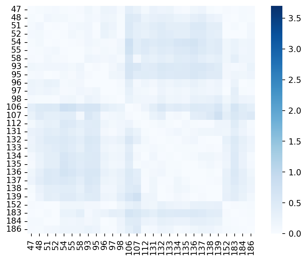

Figure 7: Comparison of distinct binding site conformations (4cwe,1uyd) using a CA distance matrix

I used the same color scale as on Figure 5 on purpose, just to have something slightly comparable (visually). However, if you look in more detail, you’ll notice that there are differences (around 0.7A max) between parts of the binding site. But obviously, they are less drastic conformational changes than what we observed before with the comparison of 3t0z & 4cwr.

Last example that I wanted to check is the impact on such a matrix of the closed conformation of the binding site. This is structure 7l7j which was already displayed in red in Figure 2 before.

Code

filename="pdbs/7l7j_aligned.pdb"
u = mda.Universe(filename)
residues = u.select_atoms('protein and chainID A and name CA and resnum {}'.format(' '.join(map(str, residue_seqnums))))
distances7l7j = distances.distance_array(residues.positions, residues.positions)

distancematrix=np.abs(distances4cwr-distances7l7j)
sns.heatmap(distancematrix,yticklabels=residue_seqnums,xticklabels=residue_seqnums,cmap="Blues",square=True)
plt.show()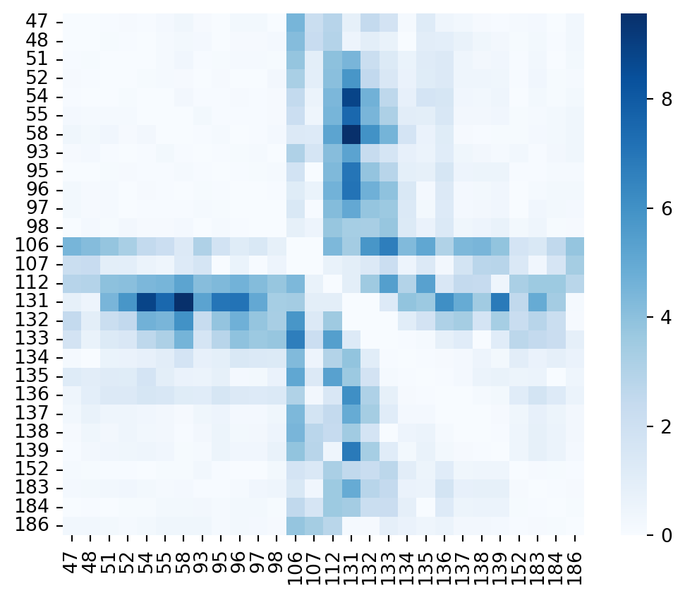

Figure 8: Comparison of distinct binding site conformations (4cwe,7l7j) using a CA distance matrix

In the figure above I didn’t set a maximum to the color scale. This way you can see the full extent of movements observed especially around residue 112 - 133. Again, let’s repeat the exercise and plot the residues that appear to be significantly moving here: 106,112, 131-133

Code

// Create drawing area
divNGL4 = html`<div style="width:800px;height:600px;position:relative"></div>`;

Figure 9: Comparison of distinct binding site conformations (4cwr, 7l7j) on specific residues

Code

stage4 = new NGL.Stage(divNGL4, { backgroundColor: "black",cameraType: "orthographic"});

pdbString42 = await FileAttachment("pdbs/4cwr_aligned.pdb").blob();
structure42 = await stage4.loadFile(pdbString42, {ext: "pdb", asTrajectory: false});
structure42.addRepresentation("trace",{ "sele": "protein", "color": "#B69849"});

Code

structure42.addRepresentation("ball+stick",{ "sele": "(106 or 112 or 131-133) and .CA", "color": "#B69849"});

Code

structure42.addRepresentation("label", {"sele": "(106 or 112 or 131-133) and .CA", "labelType":"resno", "color": "#FFEBB8"});

Code

pdbString41 = await FileAttachment("pdbs/7l7j_aligned.pdb").blob();
structure41 = await stage4.loadFile(pdbString41, {ext: "pdb", asTrajectory: false});
structure41.addRepresentation("trace",{ "sele": "protein", "color": "#B66049"});

Code

structure41.addRepresentation("ball+stick",{ "sele": "(106 or 112 or 131-133) and .CA and :A", "color": "#B66049"});

Code

structure41.addRepresentation("label", {"sele": "(106 or 112 or 131-133) and .CA and :A", "labelType":"resno", "color": "#FFC7B8"});

Code

structure41.autoView("(106 or 112 or 131-133) and .CA and :A");

The conformational changes are very important (as expected). Furthermore the selection of residues one could extract from the distance matrix is relevant also versus what can be observed above.

Clustering contact (distance) matrices

Now, in order to know whether one structure is close to another we can use these contact matrices calculated before & compare these one to another. The comparison between 4cwr & 3t0z results in a contact difference matrix (Figure 5). The comparison of 4cwr and 1uyd results in another contact difference matrix (Figure 7). Let’s try to compute an average of all the values of each contact difference matrix and see what we get.

Code

distanceMatrixList=[distances4cwr,distances3t0z,distances1uyd,distances7l7j]
labels=["4cwr","3t0z","1uyd","7l7j"]
nMatrices=len(distanceMatrixList)

result=np.zeros((nMatrices,nMatrices))
for i in range(nMatrices):
  for j in range(nMatrices):
    if i==j:
      result[i][j]=0.0
    elif i<j:
      result[i][j]=np.mean(np.abs(distanceMatrixList[i]-distanceMatrixList[j]))
      result[j][i]=result[i][j]

sns.heatmap(result,yticklabels=labels,xticklabels=labels,cmap="Blues",square=True)
plt.show()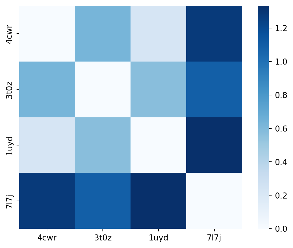

Figure 10: Comparison of distinct binding sites for clustering

That looks already rather promising. We expect to see 4cwr & 1uyd to be close to each other, and 3t0z to be closer to 4cwr than to 7l7j. However, 7l7j is not close to any of the other structures and likely closest to 3t0z (as both have the helical unfolding around residues 107-112). Now we have a distance matrix that we can feed into a clustering algorithm. I’m not a big fan of k-means as I don’t know how many clusters I expect beforehand. In the end I want the dataset preparation steps I’m going through here to be as automated as possible. So I’ll use a hierarchical clustering algorithm instead.

Code

import scipy
import scipy.spatial.distance as ssd
distArray = ssd.squareform(result)

clusters=scipy.cluster.hierarchy.linkage(distArray, method='single', metric='euclidean')
scipy.cluster.hierarchy.dendrogram(clusters,labels=labels,leaf_rotation=90)
plt.show()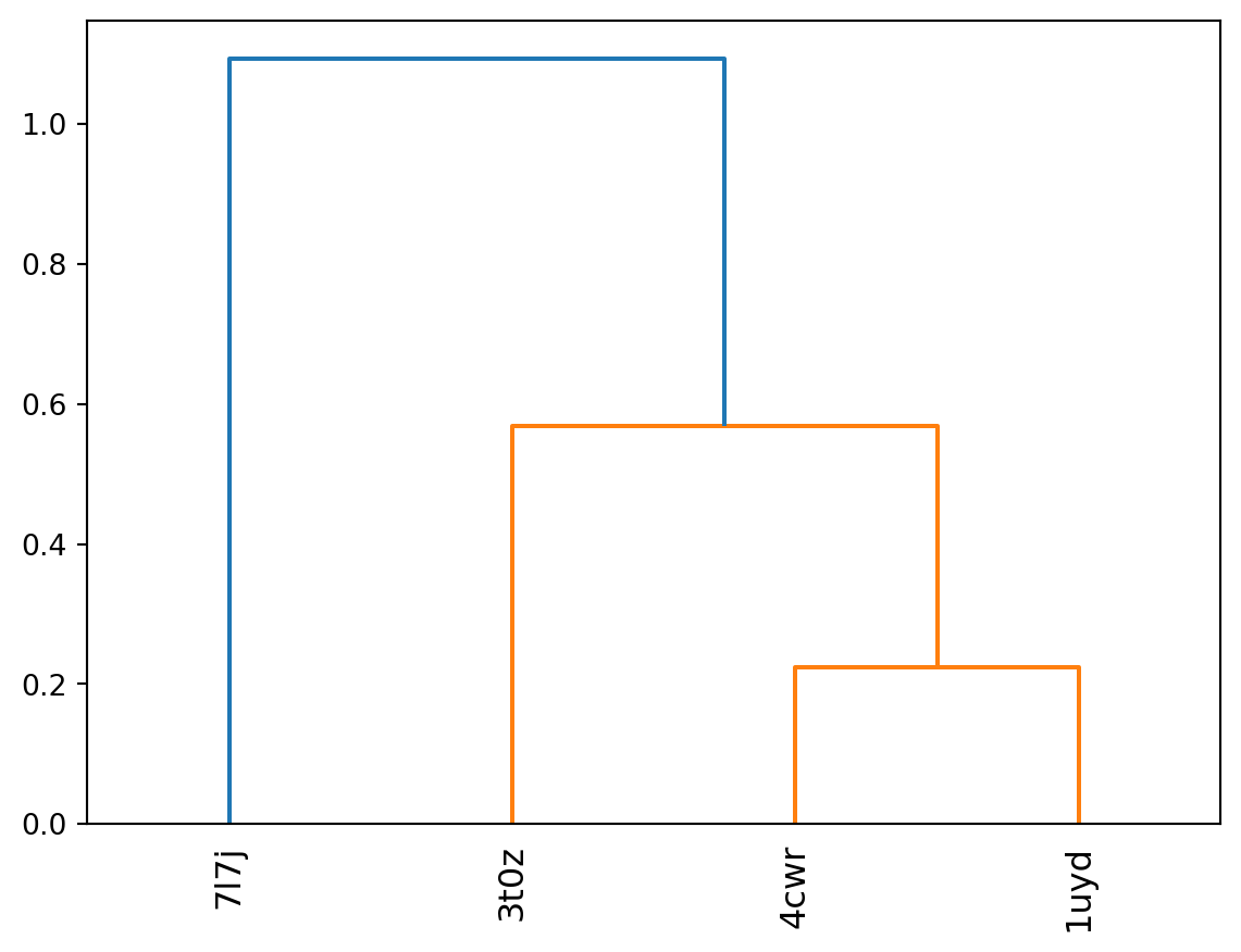

Figure 11: Dendrogram from single linkage clustering of previous distance matrix

Now that I have this, I can cut the result at any given distance and get the clusters. Obviously this example is a bit too tiny to draw any interesting insights. So in order to get ready for our first full dataset, we need to repeat the whole process for all the structures we’ve identified earlier. In order to do so I first need to properly address two items on my todo list that I tracked as side notes in the previous sections (I’ll put it here again as reference).

Things to keep in mind

• Uniprot accession vs polymer entity group ID handling to be clarified with RCSB folks
• Don’t forget to check if all sidechains of the binding site are resolved in the selected structures
• Treat homo-multimers rationally in the data-set construction
• Handle canonical residue numbering properly in distanceMatrix code
• Consider also optional side-chain sensitive distance calculations
• What to do with large motions implicating new residues in binding sites?

1. I need to verify that all structures have a canonical uniprot sequence residue numbering. If not I need to map the residue numbers to the canonical uniprot sequence.
2. I need to know which chain I use beforehand (7l7j contains two different proteins for instance - so just sticking without a selection is not an option)

Automating things

The first issue previously mentioned was briefly checked against 3decision. In the case of the selected HSP90 structures and this binding site, it’s not an issue to perform residue selections using the residue numbers I used here. You could extract that kind of info using a graphQL query from the RCSB as well, but I’ll pass here and will come back to that if / when needed. In order to address the second of the previously mentioned issues I am going to adjust a bit the graphQL query I used earlier and track for each structure which chain corresponds to HSP90 containing the binding site we are interested in here.

Code

# here we can reuse the already retrieved data from the GraphQL query that we did earlier against the RCSB, because it already contains the information we need.

# a bit of rewrite of the function we had before (still very ugly, feel free to make it pretty ;) 

def extractSequenceRegionsAndChains(data):
  result={}
  
  for entry in data:  
    result[entry["rcsb_id"]]=[]
    for entity in entry["polymer_entities"]:
      # print(entity["rcsb_polymer_entity_container_identifiers"])
      if entity["entity_poly"]["rcsb_mutation_count"]==0:
        chain_ids=entity["rcsb_polymer_entity_container_identifiers"]["auth_asym_ids"]
        for idx,identifier in enumerate(entity["rcsb_polymer_entity_container_identifiers"]["reference_sequence_identifiers"]):
          if identifier["database_name"]=="UniProt" and identifier["database_accession"]=="P07900":
            if entity["rcsb_polymer_entity_align"][idx]["reference_database_name"]=="UniProt":
              for region in entity["rcsb_polymer_entity_align"][idx]["aligned_regions"]:
                result[entry["rcsb_id"]].append((region["ref_beg_seq_id"],region["ref_beg_seq_id"]+region["length"]))
                result[entry["rcsb_id"]].append(chain_ids)
  return result

# residuelist=[47,48,51,52,54,55,58,93,95,96,97,98,106,107,112,131,132,133,134,135,136,137,138,139,152,183,184,186]


resolved_regions=extractSequenceRegionsAndChains(dataRCSBGQL)

selectedPdbCodesAndChains=[]
for pdbCode in resolved_regions:
  mapping = resolved_regions[pdbCode]
  if(len(mapping)>0 and all(i>=mapping[0][0] and i<=mapping[0][1] for i in residuelist)):
    selectedPdbCodesAndChains.append({"pdbCode":pdbCode,"chain":mapping[1][0]})

print(selectedPdbCodesAndChains)
# print(str(len(selectedPdbCodes)) + " structures identified")

[{'pdbCode': '1BYQ', 'chain': 'A'}, {'pdbCode': '1OSF', 'chain': 'A'}, {'pdbCode': '1UY6', 'chain': 'A'}, {'pdbCode': '1UY7', 'chain': 'A'}, {'pdbCode': '1UY8', 'chain': 'A'}, {'pdbCode': '1UY9', 'chain': 'A'}, {'pdbCode': '1UYC', 'chain': 'A'}, {'pdbCode': '1UYD', 'chain': 'A'}, {'pdbCode': '1UYE', 'chain': 'A'}, {'pdbCode': '1UYF', 'chain': 'A'}, {'pdbCode': '1UYG', 'chain': 'A'}, {'pdbCode': '1UYH', 'chain': 'A'}, {'pdbCode': '1UYI', 'chain': 'A'}, {'pdbCode': '1UYK', 'chain': 'A'}, {'pdbCode': '1UYL', 'chain': 'A'}, {'pdbCode': '1YC1', 'chain': 'A'}, {'pdbCode': '1YC3', 'chain': 'A'}, {'pdbCode': '1YC4', 'chain': 'A'}, {'pdbCode': '1YER', 'chain': 'A'}, {'pdbCode': '1YES', 'chain': 'A'}, {'pdbCode': '1YET', 'chain': 'A'}, {'pdbCode': '2BSM', 'chain': 'A'}, {'pdbCode': '2BT0', 'chain': 'A'}, {'pdbCode': '2BYH', 'chain': 'A'}, {'pdbCode': '2BYI', 'chain': 'A'}, {'pdbCode': '2BZ5', 'chain': 'A'}, {'pdbCode': '2CCS', 'chain': 'A'}, {'pdbCode': '2CCT', 'chain': 'A'}, {'pdbCode': '2CCU', 'chain': 'A'}, {'pdbCode': '2FWY', 'chain': 'A'}, {'pdbCode': '2FWZ', 'chain': 'A'}, {'pdbCode': '2H55', 'chain': 'A'}, {'pdbCode': '2JJC', 'chain': 'A'}, {'pdbCode': '2K5B', 'chain': 'A'}, {'pdbCode': '2QF6', 'chain': 'A'}, {'pdbCode': '2QFO', 'chain': 'A'}, {'pdbCode': '2QG0', 'chain': 'A'}, {'pdbCode': '2QG2', 'chain': 'A'}, {'pdbCode': '2UWD', 'chain': 'A'}, {'pdbCode': '2VCI', 'chain': 'A'}, {'pdbCode': '2VCJ', 'chain': 'A'}, {'pdbCode': '2WI1', 'chain': 'A'}, {'pdbCode': '2WI2', 'chain': 'A'}, {'pdbCode': '2WI3', 'chain': 'A'}, {'pdbCode': '2WI4', 'chain': 'A'}, {'pdbCode': '2WI5', 'chain': 'A'}, {'pdbCode': '2WI6', 'chain': 'A'}, {'pdbCode': '2WI7', 'chain': 'A'}, {'pdbCode': '2XAB', 'chain': 'A'}, {'pdbCode': '2XDK', 'chain': 'A'}, {'pdbCode': '2XDL', 'chain': 'A'}, {'pdbCode': '2XDS', 'chain': 'A'}, {'pdbCode': '2XDU', 'chain': 'A'}, {'pdbCode': '2XDX', 'chain': 'A'}, {'pdbCode': '2XHR', 'chain': 'A'}, {'pdbCode': '2XHT', 'chain': 'A'}, {'pdbCode': '2XHX', 'chain': 'A'}, {'pdbCode': '2XJG', 'chain': 'A'}, {'pdbCode': '2XJJ', 'chain': 'A'}, {'pdbCode': '2XJX', 'chain': 'A'}, {'pdbCode': '2XK2', 'chain': 'A'}, {'pdbCode': '2YE2', 'chain': 'A'}, {'pdbCode': '2YE3', 'chain': 'A'}, {'pdbCode': '2YE4', 'chain': 'A'}, {'pdbCode': '2YE5', 'chain': 'A'}, {'pdbCode': '2YE6', 'chain': 'A'}, {'pdbCode': '2YE7', 'chain': 'A'}, {'pdbCode': '2YE8', 'chain': 'A'}, {'pdbCode': '2YE9', 'chain': 'A'}, {'pdbCode': '2YEA', 'chain': 'A'}, {'pdbCode': '2YEB', 'chain': 'A'}, {'pdbCode': '2YEC', 'chain': 'A'}, {'pdbCode': '2YED', 'chain': 'A'}, {'pdbCode': '2YEE', 'chain': 'A'}, {'pdbCode': '2YEF', 'chain': 'A'}, {'pdbCode': '2YEG', 'chain': 'A'}, {'pdbCode': '2YEH', 'chain': 'A'}, {'pdbCode': '2YEI', 'chain': 'A'}, {'pdbCode': '2YEJ', 'chain': 'A'}, {'pdbCode': '2YI0', 'chain': 'A'}, {'pdbCode': '2YI5', 'chain': 'A'}, {'pdbCode': '2YI6', 'chain': 'A'}, {'pdbCode': '2YI7', 'chain': 'A'}, {'pdbCode': '2YJW', 'chain': 'A'}, {'pdbCode': '2YJX', 'chain': 'A'}, {'pdbCode': '2YK2', 'chain': 'A'}, {'pdbCode': '2YK9', 'chain': 'A'}, {'pdbCode': '2YKB', 'chain': 'A'}, {'pdbCode': '2YKC', 'chain': 'A'}, {'pdbCode': '2YKE', 'chain': 'A'}, {'pdbCode': '2YKI', 'chain': 'A'}, {'pdbCode': '2YKJ', 'chain': 'A'}, {'pdbCode': '3B24', 'chain': 'A'}, {'pdbCode': '3B25', 'chain': 'A'}, {'pdbCode': '3B26', 'chain': 'A'}, {'pdbCode': '3B27', 'chain': 'A'}, {'pdbCode': '3B28', 'chain': 'A'}, {'pdbCode': '3BM9', 'chain': 'A'}, {'pdbCode': '3BMY', 'chain': 'A'}, {'pdbCode': '3D0B', 'chain': 'A'}, {'pdbCode': '3EKO', 'chain': 'A'}, {'pdbCode': '3EKR', 'chain': 'A'}, {'pdbCode': '3FT5', 'chain': 'A'}, {'pdbCode': '3FT8', 'chain': 'A'}, {'pdbCode': '3HEK', 'chain': 'A'}, {'pdbCode': '3HHU', 'chain': 'A'}, {'pdbCode': '3HYY', 'chain': 'A'}, {'pdbCode': '3HYZ', 'chain': 'A'}, {'pdbCode': '3HZ1', 'chain': 'A'}, {'pdbCode': '3HZ5', 'chain': 'A'}, {'pdbCode': '3INW', 'chain': 'A'}, {'pdbCode': '3INX', 'chain': 'A'}, {'pdbCode': '3K97', 'chain': 'A'}, {'pdbCode': '3K98', 'chain': 'A'}, {'pdbCode': '3K99', 'chain': 'A'}, {'pdbCode': '3MNR', 'chain': 'P'}, {'pdbCode': '3O0I', 'chain': 'A'}, {'pdbCode': '3OW6', 'chain': 'A'}, {'pdbCode': '3OWB', 'chain': 'A'}, {'pdbCode': '3OWD', 'chain': 'A'}, {'pdbCode': '3QDD', 'chain': 'A'}, {'pdbCode': '3QTF', 'chain': 'A'}, {'pdbCode': '3R4M', 'chain': 'A'}, {'pdbCode': '3R4N', 'chain': 'A'}, {'pdbCode': '3R4O', 'chain': 'A'}, {'pdbCode': '3R4P', 'chain': 'A'}, {'pdbCode': '3R91', 'chain': 'A'}, {'pdbCode': '3R92', 'chain': 'A'}, {'pdbCode': '3RKZ', 'chain': 'A'}, {'pdbCode': '3RLP', 'chain': 'A'}, {'pdbCode': '3RLQ', 'chain': 'A'}, {'pdbCode': '3RLR', 'chain': 'A'}, {'pdbCode': '3T0H', 'chain': 'A'}, {'pdbCode': '3T0Z', 'chain': 'A'}, {'pdbCode': '3T10', 'chain': 'A'}, {'pdbCode': '3T1K', 'chain': 'A'}, {'pdbCode': '3T2S', 'chain': 'A'}, {'pdbCode': '3TUH', 'chain': 'A'}, {'pdbCode': '3VHA', 'chain': 'A'}, {'pdbCode': '3VHC', 'chain': 'A'}, {'pdbCode': '3VHD', 'chain': 'A'}, {'pdbCode': '3WHA', 'chain': 'A'}, {'pdbCode': '3WQ9', 'chain': 'A'}, {'pdbCode': '4AWO', 'chain': 'A'}, {'pdbCode': '4AWP', 'chain': 'A'}, {'pdbCode': '4AWQ', 'chain': 'A'}, {'pdbCode': '4B7P', 'chain': 'A'}, {'pdbCode': '4BQG', 'chain': 'A'}, {'pdbCode': '4BQJ', 'chain': 'A'}, {'pdbCode': '4CWF', 'chain': 'A'}, {'pdbCode': '4CWN', 'chain': 'A'}, {'pdbCode': '4CWO', 'chain': 'A'}, {'pdbCode': '4CWP', 'chain': 'A'}, {'pdbCode': '4CWQ', 'chain': 'A'}, {'pdbCode': '4CWR', 'chain': 'A'}, {'pdbCode': '4CWS', 'chain': 'A'}, {'pdbCode': '4CWT', 'chain': 'A'}, {'pdbCode': '4EEH', 'chain': 'A'}, {'pdbCode': '4EFT', 'chain': 'A'}, {'pdbCode': '4EFU', 'chain': 'A'}, {'pdbCode': '4EGH', 'chain': 'A'}, {'pdbCode': '4EGI', 'chain': 'A'}, {'pdbCode': '4EGK', 'chain': 'A'}, {'pdbCode': '4FCP', 'chain': 'A'}, {'pdbCode': '4FCQ', 'chain': 'A'}, {'pdbCode': '4FCR', 'chain': 'A'}, {'pdbCode': '4HY6', 'chain': 'A'}, {'pdbCode': '4JQL', 'chain': 'A'}, {'pdbCode': '4L8Z', 'chain': 'A'}, {'pdbCode': '4L90', 'chain': 'A'}, {'pdbCode': '4L91', 'chain': 'A'}, {'pdbCode': '4L93', 'chain': 'A'}, {'pdbCode': '4L94', 'chain': 'A'}, {'pdbCode': '4LWE', 'chain': 'A'}, {'pdbCode': '4LWF', 'chain': 'A'}, {'pdbCode': '4LWG', 'chain': 'A'}, {'pdbCode': '4LWH', 'chain': 'A'}, {'pdbCode': '4LWI', 'chain': 'A'}, {'pdbCode': '4NH7', 'chain': 'A'}, {'pdbCode': '4NH8', 'chain': 'A'}, {'pdbCode': '4O04', 'chain': 'A'}, {'pdbCode': '4O05', 'chain': 'A'}, {'pdbCode': '4O07', 'chain': 'A'}, {'pdbCode': '4O09', 'chain': 'A'}, {'pdbCode': '4O0B', 'chain': 'A'}, {'pdbCode': '4R3M', 'chain': 'A'}, {'pdbCode': '4U93', 'chain': 'A'}, {'pdbCode': '4W7T', 'chain': 'A'}, {'pdbCode': '4XIP', 'chain': 'A'}, {'pdbCode': '4XIQ', 'chain': 'A'}, {'pdbCode': '4XIR', 'chain': 'A'}, {'pdbCode': '4XIT', 'chain': 'A'}, {'pdbCode': '4YKQ', 'chain': 'A'}, {'pdbCode': '4YKR', 'chain': 'A'}, {'pdbCode': '4YKT', 'chain': 'A'}, {'pdbCode': '4YKU', 'chain': 'A'}, {'pdbCode': '4YKW', 'chain': 'A'}, {'pdbCode': '4YKX', 'chain': 'A'}, {'pdbCode': '4YKY', 'chain': 'A'}, {'pdbCode': '4YKZ', 'chain': 'A'}, {'pdbCode': '5CF0', 'chain': 'A'}, {'pdbCode': '5FNC', 'chain': 'A'}, {'pdbCode': '5FND', 'chain': 'A'}, {'pdbCode': '5FNF', 'chain': 'A'}, {'pdbCode': '5GGZ', 'chain': 'A'}, {'pdbCode': '5J20', 'chain': 'A'}, {'pdbCode': '5J27', 'chain': 'A'}, {'pdbCode': '5J2V', 'chain': 'A'}, {'pdbCode': '5J2X', 'chain': 'A'}, {'pdbCode': '5J64', 'chain': 'A'}, {'pdbCode': '5J6L', 'chain': 'A'}, {'pdbCode': '5J6M', 'chain': 'A'}, {'pdbCode': '5J6N', 'chain': 'A'}, {'pdbCode': '5J82', 'chain': 'A'}, {'pdbCode': '5J86', 'chain': 'A'}, {'pdbCode': '5J8M', 'chain': 'A'}, {'pdbCode': '5J8U', 'chain': 'A'}, {'pdbCode': '5J9X', 'chain': 'A'}, {'pdbCode': '5LNY', 'chain': 'A'}, {'pdbCode': '5LNZ', 'chain': 'A'}, {'pdbCode': '5LO0', 'chain': 'A'}, {'pdbCode': '5LO1', 'chain': 'A'}, {'pdbCode': '5LO5', 'chain': 'A'}, {'pdbCode': '5LO6', 'chain': 'A'}, {'pdbCode': '5LQ9', 'chain': 'A'}, {'pdbCode': '5LR1', 'chain': 'A'}, {'pdbCode': '5LR7', 'chain': 'A'}, {'pdbCode': '5LRL', 'chain': 'A'}, {'pdbCode': '5LRZ', 'chain': 'A'}, {'pdbCode': '5LS1', 'chain': 'A'}, {'pdbCode': '5M4E', 'chain': 'A'}, {'pdbCode': '5M4H', 'chain': 'A'}, {'pdbCode': '5NYH', 'chain': 'A'}, {'pdbCode': '5NYI', 'chain': 'A'}, {'pdbCode': '5OCI', 'chain': 'A'}, {'pdbCode': '5OD7', 'chain': 'A'}, {'pdbCode': '5ODX', 'chain': 'A'}, {'pdbCode': '5T21', 'chain': 'A'}, {'pdbCode': '5VYY', 'chain': 'A'}, {'pdbCode': '5XQD', 'chain': 'A'}, {'pdbCode': '5XQE', 'chain': 'A'}, {'pdbCode': '5XR5', 'chain': 'A'}, {'pdbCode': '5XR9', 'chain': 'A'}, {'pdbCode': '5XRB', 'chain': 'A'}, {'pdbCode': '5XRD', 'chain': 'A'}, {'pdbCode': '5XRE', 'chain': 'A'}, {'pdbCode': '5ZR3', 'chain': 'A'}, {'pdbCode': '6B99', 'chain': 'A'}, {'pdbCode': '6B9A', 'chain': 'A'}, {'pdbCode': '6CEO', 'chain': 'A'}, {'pdbCode': '6CYG', 'chain': 'A'}, {'pdbCode': '6CYH', 'chain': 'A'}, {'pdbCode': '6EI5', 'chain': 'A'}, {'pdbCode': '6EL5', 'chain': 'A'}, {'pdbCode': '6ELN', 'chain': 'A'}, {'pdbCode': '6ELO', 'chain': 'A'}, {'pdbCode': '6ELP', 'chain': 'A'}, {'pdbCode': '6EY8', 'chain': 'A'}, {'pdbCode': '6EY9', 'chain': 'A'}, {'pdbCode': '6EYA', 'chain': 'A'}, {'pdbCode': '6EYB', 'chain': 'A'}, {'pdbCode': '6F1N', 'chain': 'A'}, {'pdbCode': '6FCJ', 'chain': 'A'}, {'pdbCode': '6GPR', 'chain': 'A'}, {'pdbCode': '6GPT', 'chain': 'A'}, {'pdbCode': '6GPW', 'chain': 'A'}, {'pdbCode': '6GPY', 'chain': 'A'}, {'pdbCode': '6GQ6', 'chain': 'A'}, {'pdbCode': '6GQR', 'chain': 'A'}, {'pdbCode': '6HHR', 'chain': 'A'}, {'pdbCode': '6LR9', 'chain': 'A'}, {'pdbCode': '6LSZ', 'chain': 'A'}, {'pdbCode': '6LT8', 'chain': 'A'}, {'pdbCode': '6LTI', 'chain': 'A'}, {'pdbCode': '6LTK', 'chain': 'A'}, {'pdbCode': '6N8X', 'chain': 'A'}, {'pdbCode': '6TN4', 'chain': 'AAA'}, {'pdbCode': '6TN5', 'chain': 'AAA'}, {'pdbCode': '6U99', 'chain': 'A'}, {'pdbCode': '6U9B', 'chain': 'A'}, {'pdbCode': '7DMC', 'chain': 'A'}, {'pdbCode': '7KRJ', 'chain': 'A'}, {'pdbCode': '7KW7', 'chain': 'A'}, {'pdbCode': '7L7I', 'chain': 'A'}, {'pdbCode': '7L7J', 'chain': 'A'}, {'pdbCode': '7LSZ', 'chain': 'A'}, {'pdbCode': '7LT0', 'chain': 'A'}, {'pdbCode': '7S8Y', 'chain': 'A'}, {'pdbCode': '7S8Z', 'chain': 'A'}, {'pdbCode': '7S90', 'chain': 'A'}, {'pdbCode': '7S95', 'chain': 'A'}, {'pdbCode': '7S98', 'chain': 'A'}, {'pdbCode': '7S99', 'chain': 'A'}, {'pdbCode': '7S9F', 'chain': 'A'}, {'pdbCode': '7S9G', 'chain': 'A'}, {'pdbCode': '7S9H', 'chain': 'A'}, {'pdbCode': '7S9I', 'chain': 'A'}, {'pdbCode': '7UR3', 'chain': 'A'}, {'pdbCode': '8AGI', 'chain': 'A'}]

Now we have the list of pdb codes & the chain we need to use here. Let’s wrap up the rest of the whole process to produce a larger distance matrix & clustering result. In the list of pdb codes above, several structures are NOT anymore available in the PDB format. So I have to adapt the previous code to work with mmCIF files instead. And lucky as I am, MDanalysis doesn’t seem to support them very well, nor mmtf which apparently doesn’t read in chain information from mmCIF files. So I’ll have to rewrite all of that using a different toolkit closer to crystallographers, i.e. gemmi.

from gemmi import cif
import urllib

pdbCode="3t0z"
chainCode="A"
content= urllib.request.urlopen("https://files.rcsb.org/view/"+pdbCode+".cif").read()

block=cif.read_string(content)[0]
structure=gemmi.make_structure_from_block(block)

positions=[]
for model in structure:
  for chain in model:
    if chain.name == chainCode:
      for residue in chain:
        if residue.seqid.num in residuelist:
          for atom in residue:
            if atom.name=="CA":
              positions.append(atom.pos.tolist())

if(len(positions)!=len(residuelist)):
  print("Not all positions found")
  print("stopping here")

positions_np=np.array(positions)
distances3t0zgemmi = cdist(positions_np, positions_np, 'euclidean')
if(np.all(distances3t0z-distances3t0zgemmi<0.0001)):
  print("distances match with previous analysis")
else:
  print("distances don't match with previous analysis")

distances match with previous analysis

Things to keep in mind

• Uniprot accession vs polymer entity group ID handling to be clarified with RCSB folks
• Don’t forget to check if all sidechains of the binding site are resolved in the selected structures
• Treat homo-multimers rationally in the data-set construction
• Handle canonical residue numbering properly in distanceMatrix code
• Consider also optional side-chain sensitive distance calculations
• What to do with large motions implicating new residues in binding sites?
• Decide how to handle NMR conformations in the dataset

In the code snippet above I’m checking if the results we obtained with the horrible quadruple loop match the results we got earlier with MDAnalysis on the same structure. This appears to be the case here.

Now let’s put the whole thing into a function, loop over all our structures & I guess adjust what needs adjustments (as for sure I’ll have something that will fail 😫). By the time of the writing 4 structures were found to have 1 residue implicated in the binding site to be not resolved. They’ll be discarded from further analyses.

Code

def getContactMatrix(pdbCode, chainCode, residueSelection, debug=False):
  content= urllib.request.urlopen("https://files.rcsb.org/view/"+pdbCode+".cif").read()

  block=cif.read_string(content)[0]
  structure=gemmi.make_structure_from_block(block)

  positions=[]
  for model in structure:
    if model.name=="1":
      for chain in model:
        if chain.name == chainCode:
          for residue in chain:
            if residue.seqid.num in residueSelection:
              if debug: print(residue.seqid.num)
              for atom in residue:
                if atom.name=="CA":
                  if debug: print("ok")
                  positions.append(atom.pos.tolist())
                  break #we need that for multiple occurences

  if(len(positions)!=len(residueSelection)):
    print("Not all positions found for "+pdbCode+" discarding structure")
    return None

  positions_np=np.array(positions)
  return cdist(positions_np, positions_np, 'euclidean')

def clusterMatrices(matrixList):  
  nMatrices=len(matrixList)
  result=np.zeros((nMatrices,nMatrices))
  for i in range(nMatrices):
    for j in range(nMatrices):
      if i==j:
        result[i][j]=0.0
      elif i<j:
        result[i][j]=np.mean(np.abs(matrixList[i]-matrixList[j]))
        result[j][i]=result[i][j]

  
  distArray = ssd.squareform(result)
  clusters=scipy.cluster.hierarchy.linkage(result, method='single', metric='euclidean')
  return(clusters)


contactMatrices=[getContactMatrix(structure["pdbCode"],structure["chain"],residuelist) for structure in selectedPdbCodesAndChains]

none_indices = [ic for ic, matrix in enumerate(contactMatrices) if matrix is None]

labels=[structure["pdbCode"] for structure in selectedPdbCodesAndChains]
chainCodes=[structure["chain"] for structure in selectedPdbCodesAndChains]
filteredContactMatrices = [matrix for i, matrix in enumerate(contactMatrices) if i not in none_indices]

filteredLabels = [label for idx, label in enumerate(labels) if idx not in none_indices]
filteredChainCodes= [code for idx, code in enumerate(chainCodes) if idx not in none_indices]

clusters=clusterMatrices(filteredContactMatrices)

plt.figure(figsize=(10, 40))

scipy.cluster.hierarchy.dendrogram(clusters,labels=filteredLabels,orientation='right',leaf_font_size=7,color_threshold=1.0)
plt.show()

Not all positions found for 2YI5 discarding structure
Not all positions found for 3HYZ discarding structure
Not all positions found for 4FCR discarding structure
Not all positions found for 6EYA discarding structure

/var/folders/51/p06ylvs507q40bm1kxbl65km0000gp/T/ipykernel_94855/1742338535.py:41: ClusterWarning:

scipy.cluster: The symmetric non-negative hollow observation matrix looks suspiciously like an uncondensed distance matrix

Figure 12: Result of hierarchical clustering of HSP90 ATP binding sites based on CA positions

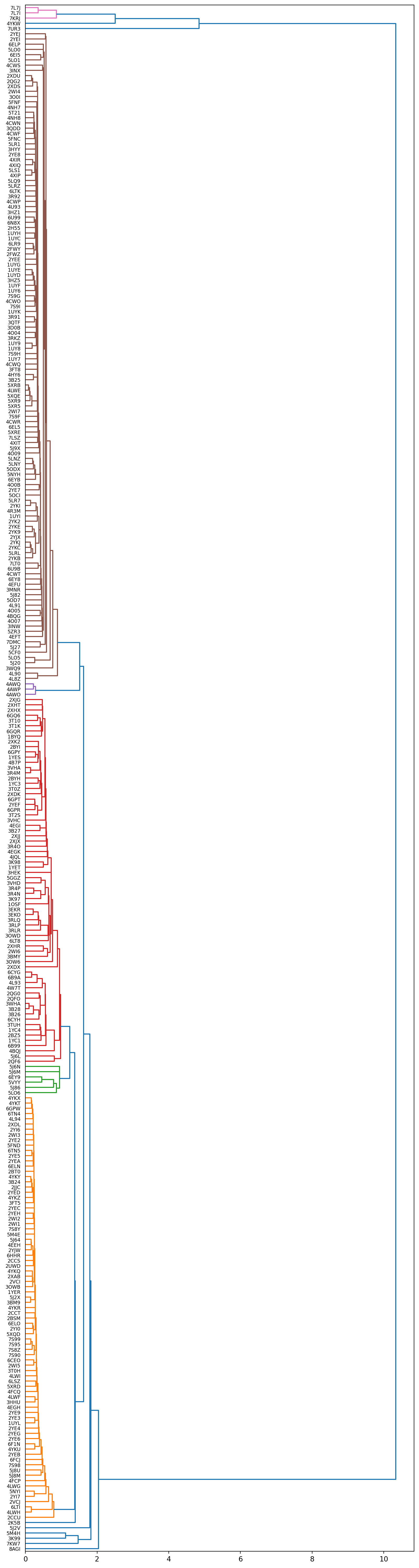
Alright, this is starting to look like something useable. The colors encode clusters, when cutting the dendrogram at a distance of 1.0 we get 3 very large clusters and several smaller ones & outliers.

Let’s cherrypick 2 structures from each of the 3 large clusters and see if we can observe structural reasons underlinging these results:

Code

// Create drawing area
divNGL5 = html`<div style="width:800px;height:600px;position:relative"></div>`;

Figure 13: Comparison of 2 representative binding sites for each of the 3 large clusters identified. Orange, 2 structures from the orange cluster of Figure 12; red, 2 structures from the red cluster of Figure 12; blue, 2 structures from the brown cluster of Figure 12.

Code

stage5 = new NGL.Stage(divNGL5, { backgroundColor: "black",cameraType: "orthographic"});
{
  let files=[await FileAttachment("pdbs/4yku_aligned.pdb").blob(),
    await FileAttachment("pdbs/2yi6_aligned.pdb").blob(),
    await FileAttachment("pdbs/1yc4_aligned.pdb").blob(),
    await FileAttachment("pdbs/2xjg_aligned.pdb").blob(),
    await FileAttachment("pdbs/4o05_aligned.pdb").blob(),
    await FileAttachment("pdbs/2xdu_aligned.pdb").blob()]
  let colors=["#EF740E","#EF740E","#B7040D","#B7040D","#48ABAB","#48ABAB"]
  let structures=[]

  for (let [index,file] of files.entries()){
    let structure = await stage5.loadFile(file, {ext: "pdb", asTrajectory: false});
    structure.addRepresentation("ribbon",{ "radius":0.1,"sele": "protein", "color": colors[index]});
    structures.push(structure)
  };
  structures[0].autoView("(106-107 or 112 or 131-139) and .CA");
}

In the 3D View we can nicely see that we clustered the different conformations that occur for the majority of HSP90 alpha human structures in the PDB.

Code

from scipy.cluster.hierarchy import cut_tree
h_cluster_id = cut_tree(clusters, height=1.0).reshape(-1, )
sns.displot(h_cluster_id)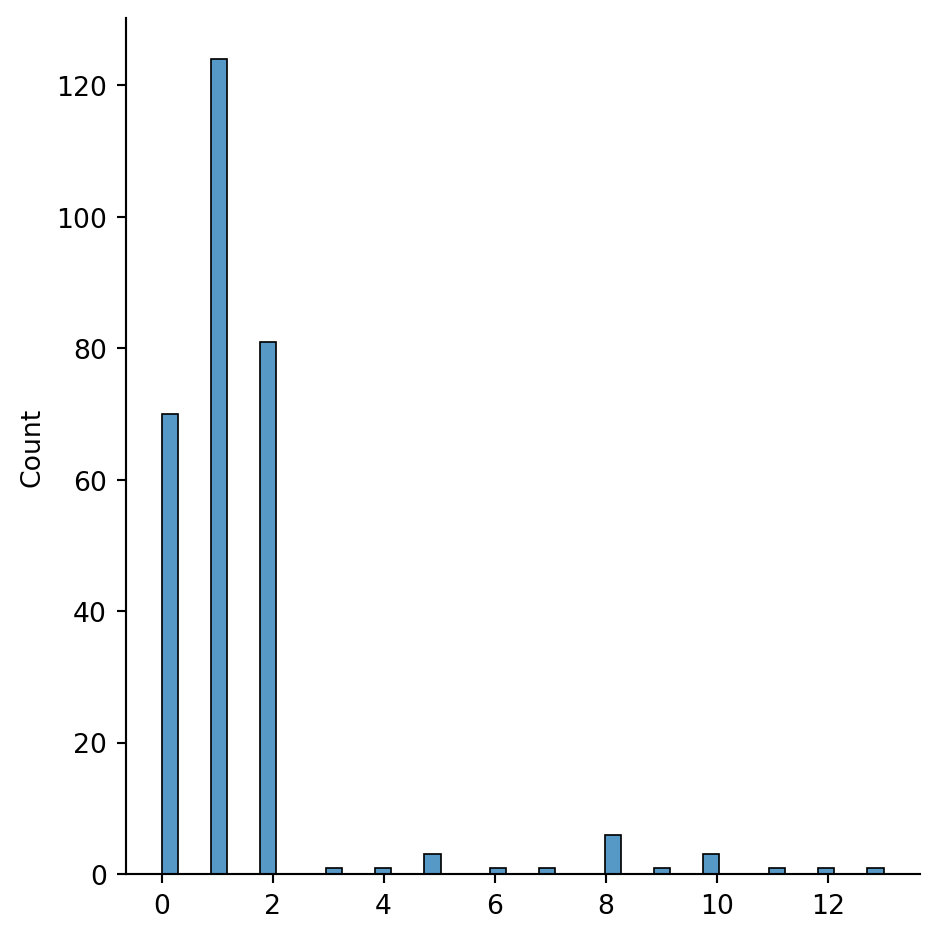

Figure 14: Size distribution of identified clusters (cut at 1A distance).

The histogram above here shows nicely these 3 larger groups and the rest. Obviously we can play around with where do we cut the dendrogram to get more or less clusters. However, here I’ll rather stick to the current cut at 1A. We can revise that at a later stage if needed.

Wrap-up

Well that got more complicated than it should have been, didn’t it? And unfortunately that was the easy part. Now we can extend the set gradually 🎉.

But let’s resume a bit what can be done with these results & scripts I provide here. We now have a set of structures that:

1. have been automagically selected from the PDB
2. this selection can be updated at any time (unless they change their API, which they will at some point)
3. we have performed local structure comparison to know which known ATP binding sites are similar to each other in terms of conformation

This set of structures, and especially the clusters, can be used to serve as known positives for binding site benchmarking. It can also be used to evaluate rank ordering for binding site comparison methods.

Code

from IPython.display import Markdown
from tabulate import tabulate
identifiers=["{}:{}".format(a_, b_) for a_, b_ in zip(filteredLabels, filteredChainCodes)]
table = list(zip(identifiers, h_cluster_id))
Markdown(tabulate(
  table, 
  headers=["Structure","Cluster ID"], colalign=("center","center")
))

Final List of structures and their corresponding cluster ID of the selected HSP90 alpha human ATP binding site containing structures

Structure	Cluster ID
1BYQ:A	0
1OSF:A	0
1UY6:A	1
1UY7:A	1
1UY8:A	1
1UY9:A	1
1UYC:A	1
1UYD:A	1
1UYE:A	1
1UYF:A	1
1UYG:A	1
1UYH:A	1
1UYI:A	1
1UYK:A	1
1UYL:A	2
1YC1:A	0
1YC3:A	0
1YC4:A	0
1YER:A	2
1YES:A	0
1YET:A	0
2BSM:A	2
2BT0:A	2
2BYH:A	0
2BYI:A	0
2BZ5:A	0
2CCS:A	2
2CCT:A	2
2CCU:A	2
2FWY:A	1
2FWZ:A	1
2H55:A	1
2JJC:A	2
2K5B:A	3
2QF6:A	0
2QFO:A	0
2QG0:A	0
2QG2:A	1
2UWD:A	2
2VCI:A	2
2VCJ:A	2
2WI1:A	2
2WI2:A	2
2WI3:A	2
2WI4:A	1
2WI5:A	2
2WI6:A	0
2WI7:A	1
2XAB:A	2
2XDK:A	0
2XDL:A	2
2XDS:A	1
2XDU:A	1
2XDX:A	0
2XHR:A	0
2XHT:A	0
2XHX:A	0
2XJG:A	0
2XJJ:A	0
2XJX:A	0
2XK2:A	0
2YE2:A	2
2YE3:A	2
2YE4:A	2
2YE5:A	2
2YE6:A	2
2YE7:A	1
2YE8:A	1
2YE9:A	2
2YEA:A	2
2YEB:A	2
2YEC:A	2
2YED:A	2
2YEE:A	1
2YEF:A	0
2YEG:A	2
2YEH:A	2
2YEI:A	1
2YEJ:A	1
2YI0:A	2
2YI6:A	2
2YI7:A	2
2YJW:A	2
2YJX:A	1
2YK2:A	1
2YK9:A	1
2YKB:A	1
2YKC:A	1
2YKE:A	1
2YKI:A	1
2YKJ:A	1
3B24:A	2
3B25:A	1
3B26:A	0
3B27:A	0
3B28:A	0
3BM9:A	2
3BMY:A	0
3D0B:A	1
3EKO:A	0
3EKR:A	0
3FT5:A	2
3FT8:A	1
3HEK:A	0
3HHU:A	2
3HYY:A	1
3HZ1:A	1
3HZ5:A	1
3INW:A	1
3INX:A	1
3K97:A	0
3K98:A	0
3K99:A	4
3MNR:P	1
3O0I:A	1
3OW6:A	0
3OWB:A	2
3OWD:A	0
3QDD:A	1
3QTF:A	1
3R4M:A	0
3R4N:A	0
3R4O:A	0
3R4P:A	0
3R91:A	1
3R92:A	1
3RKZ:A	1
3RLP:A	0
3RLQ:A	0
3RLR:A	0
3T0H:A	2
3T0Z:A	0
3T10:A	0
3T1K:A	0
3T2S:A	0
3TUH:A	0
3VHA:A	0
3VHC:A	0
3VHD:A	0
3WHA:A	0
3WQ9:A	1
4AWO:A	5
4AWP:A	5
4AWQ:A	5
4B7P:A	0
4BQG:A	1
4BQJ:A	0
4CWF:A	1
4CWN:A	1
4CWO:A	1
4CWP:A	1
4CWQ:A	1
4CWR:A	1
4CWS:A	1
4CWT:A	1
4EEH:A	2
4EFT:A	1
4EFU:A	1
4EGH:A	2
4EGI:A	0
4EGK:A	0
4FCP:A	2
4FCQ:A	2
4HY6:A	1
4JQL:A	0
4L8Z:A	1
4L90:A	1
4L91:A	1
4L93:A	0
4L94:A	2
4LWE:A	1
4LWF:A	2
4LWG:A	2
4LWH:A	2
4LWI:A	2
4NH7:A	1
4NH8:A	1
4O04:A	1
4O05:A	1
4O07:A	1
4O09:A	1
4O0B:A	1
4R3M:A	1
4U93:A	1
4W7T:A	0
4XIP:A	1
4XIQ:A	1
4XIR:A	1
4XIT:A	1
4YKQ:A	2
4YKR:A	2
4YKT:A	2
4YKU:A	2
4YKW:A	6
4YKX:A	2
4YKY:A	2
4YKZ:A	2
5CF0:A	1
5FNC:A	1
5FND:A	2
5FNF:A	1
5GGZ:A	0
5J20:A	1
5J27:A	1
5J2V:A	7
5J2X:A	2
5J64:A	2
5J6L:A	0
5J6M:A	8
5J6N:A	8
5J82:A	1
5J86:A	8
5J8M:A	2
5J8U:A	2
5J9X:A	1
5LNY:A	1
5LNZ:A	1
5LO0:A	1
5LO1:A	1
5LO5:A	1
5LO6:A	8
5LQ9:A	1
5LR1:A	1
5LR7:A	1
5LRL:A	1
5LRZ:A	1
5LS1:A	1
5M4E:A	2
5M4H:A	9
5NYH:A	1
5NYI:A	2
5OCI:A	1
5OD7:A	1
5ODX:A	1
5T21:A	1
5VYY:A	8
5XQD:A	2
5XQE:A	1
5XR5:A	1
5XR9:A	1
5XRB:A	1
5XRD:A	2
5XRE:A	1
5ZR3:A	1
6B99:A	0
6B9A:A	0
6CEO:A	2
6CYG:A	0
6CYH:A	0
6EI5:A	1
6EL5:A	1
6ELN:A	2
6ELO:A	2
6ELP:A	1
6EY8:A	1
6EY9:A	8
6EYB:A	1
6F1N:A	2
6FCJ:A	2
6GPR:A	0
6GPT:A	0
6GPW:A	2
6GPY:A	0
6GQ6:A	0
6GQR:A	0
6HHR:A	2
6LR9:A	1
6LSZ:A	2
6LT8:A	0
6LTI:A	2
6LTK:A	1
6N8X:A	1
6TN4:AAA	2
6TN5:AAA	2
6U99:A	1
6U9B:A	1
7DMC:A	1
7KRJ:A	10
7KW7:A	11
7L7I:A	10
7L7J:A	10
7LSZ:A	1
7LT0:A	1
7S8Y:A	2
7S8Z:A	2
7S90:A	2
7S95:A	2
7S98:A	2
7S99:A	2
7S9F:A	1
7S9G:A	1
7S9H:A	1
7S9I:A	1
7UR3:A	12
8AGI:A	13

Comparison to existing literature

This section is to verify how this very first section on very similar binding sites differs from already existing papers. The idea is to provide constructive criticism and not to bash anyone’s work - and probably I’ll have to revise a few things on my side while reading yet again into some details of some of the published work.

Prospeccts Ehrt, Brinkjost, and Koch (2018)

The first data set (structures with identical sequences) was designed to evaluate the tools’ sensitivity to the binding site definition. This definition often depends on the size and location of bound ligands. Different ligands can address various regions of the binding site of interest (sub-pockets). Because of these different site definitions, similar sub-pockets are more difficult to match. Although binding sites can interact with a broad variety of ligands, they share common properties and distinct similarities. Thus, the scoring scheme has to be optimized for this scenario to enrich similar binding site pairs with different cavity definitions in a ranked list. Data set 1 contains structures with identical sequences, which bind to chemically different ligands located at identical sites, leading to diverse binding site definitions used for the comparisons.

• First first major difference that pops up here is that the binding site appears to be defined using the ligand bound to HSP90
  • This is something I already discussed in my previous post on the drawbacks of binding site comparison benchmarks
  • No apo structures can be considered here
  • On top of structural variation one adds the variation of the definition on where the binding site exactly is
    • Ehrt, Brinkjost, and Koch (2018) et al are totally right that this is something to check. I’m just relunctant to use this to define an ideal benchmark set.
      
  • One drawback I have here is that my binding site definition is totally fixed by residue numbers. If the structure moves (i.e. residues 107-112 in HSP90) this definition might change.
• Second they cluster by identical sequence, as opposed to what I did here (same protein strictly speaking)
  • that very likely something I might revise on my side when starting with the 2nd set of structures with similar sequences on non identical proteins - but for let’s keep it clean & simple.

The sequences of all single chain entries of the sc-PDB[65] were sequence culled using the PISCES[104] server (with a sequence identity threshold of 25%). The single chain sc-PDB entry sequences of the culled set were compared to those of all single chain proteins as stored in the PDB using USEARCH[105]. Structures whose sequences were identical to those of at least nine others were retained. This resulted in a data set of 13 groups of diverse structures. The PDB structures within each group were aligned and the ligand-occupied binding sites were compared to ensure that all ligands were located at the same site. This visual inspection led to the exclusion of one group represented by the sc-PDB entry with the PDB ID 4l8u (chain A) as the ligand-defined binding sites differed for the structures with 100% sequence identity. A complete list of data set 1 can be found in S9 Table. An all-against-all comparison was performed to assess the performance of each tool. Site pairs of proteins with identical sequences were regarded as positives while other matches were defined as negatives.

• I’m a bit puzzled by the fact that they obtain only 13 groups through such an approach (that’s just a comment)
• The structures were aligned, but not sure how (cf the discussion that I had earlier) & that’s not reproducible now
• Visual inspection is ok, but not reproducible as well
• In the end we have a set with binding site locations & conformations that could potentially vary significantly (i.e. the 7l7j vs 4cwr comparison that we had in the post)
• I’m not sure I understood how the sc-PDB is used as reference or limit here (goes back to point #1 above)
• As this is not reproducible, I cannot use the approach to update a benchmark set at any time
• The approch used by the authors only considers single chain structures, which can be a limitation when you want to extend you dataset
• Again I’m not sure how the sc-PDB vs PDB query is run here and to which extent there are quality filters in there. I don’t filter at all by commonly used quality filters

APoc Gao and Skolnick (2013)

3. Bench Subject/Control Sets. Two sets are used to benchmark the performance of APoc. Complete linkage clustering was first conducted on unique ligands curated from the PDB (see above) at a Tc threshold of 0.5, which indicates a high level chemical similarity (the mean/sd of Tc is 0.16/0.12 among all ligands in the PDB). In each cluster, the ligand type most found frequently in the pockets of protein chains curated at 90% sequence identity is selected as the cluster representative, e.g. ADP represents a cluster of ligands including AMP, ATP, etc. Within each cluster, we used a graph-based algorithm, SIMCOMP (Hattori et al., 2010), to obtain the equivalence between heavy atoms of each pair of ligands. We collect atomic contacts between heavy atoms of the ligand and protein. Two ligand–protein contacts from two separate structures are of the same type if the ligand atoms are mapped each other in the SIMCOMP alignment and the protein residues belong to the same group defined above for Equation 4. We then define the Subject set as pairs of pockets such that:

• Ligands found in these two pockets have a Tc ≥ 0.5,
• Sequence similarity < 30% between the two associated proteins,
• They share ≥ 50 atomic ligand–protein contacts of same type. In total, we found 38 066 pairs of pockets for the Subject set. We expect that a significant number of entries in this set share a high level of pocket similarity because they recognize the same or similar types of ligands and likely possess a putative common anchor region due to the overlap of a large number of ligand-pocket contacts (Brylinski and Skolnick, 2009). Note that no geometric information is explicitly used in this procedure.

Well this is a totally different approach and very much focused around the “similar ligands bind to similar pockets” assumption, strengthened by the use of contact analysis. As such the dataset is not at all comparable to what we have for now, it is likely already very challenging.

Though Dataset Govindaraj and Brylinski (2018)

First, we identified in the PDB protein chains composed of 50–999 amino acids that non-covalently bind small organic molecules (“Select ligand-bound proteins”). No constraints were imposed on the resolution to maximize the coverage and include experimentally determined structures of varied quality. Next, we retained those proteins binding a single ligand whose TC to at least one FDA-approved drug is ≥0.5 (“Select drug-like molecules”). The TC is calculated for 1024-bit molecular fingerprints with OpenBabel [44] against FDA-approved drugs in the DrugBank database [45]. Subsequently, protein sequences were clustered with CD-HIT [46] at 40% sequence similarity (“Cluster proteins”). From each homologous cluster, we selected a representative set of proteins binding chemically dissimilar ligands whose pairwise TC is < 0.5 at different locations separated by at least 8 Å (“Select representative complexes”). … In the next step, all target-bound ligands were clustered with the SUBSET program [49] (“Cluster ligands”). Using a TC threshold of 0.7 produced 1266 groups of chemically similar molecules. From all possible combinations of protein pairs within each cluster of similar compounds, we selected those having a TM-score of < 0.4 as reported by Fr-TM-align [50] (“Select globally dissimilar protein pairs”). The Positive subset of TOUGH-M1 comprises 505,116 protein pairs having different structures, yet binding chemically similar ligands. Finally, we identified a representative structure within each group of proteins binding similar compounds, and considered all pairwise combinations of structures from different clusters that have a TM-score to one another of < 0.4 (“Select globally dissimilar protein pairs”). The Negative subset of TOUGH-M1 comprises 556,810 protein pairs that have different structures and bind chemically dissimilar ligands.

The approach taken to create the Tough M1 dataset is similar to the one for APoc. It’s focused on identifying positive matching binding sites using ligand similarity & structural dissimilarity as main drivers. So the conclusion is the same as for APoc, it’s not at all overlapping with what I did here.

Shaper & Fuzcav Desaphy et al. (2012) & Weill and Rognan (2010)

An sc-PDB binding site is defined by any monomer (amino acid, ion, cofactor, prosthetic group) presenting one heavy atom closer than 6.5 Å from any heavy atom of the pharmacological ligand. All protein-ligand binding sites have been retrieved from the 2008 release of the sc-PDB database, which currently comprises 5952 entries … Data set 1 is composed of 769 pairs of nonredundant similar binding sites seeded with 769 pairs of nonredundant dissimilar binding sites. The similar pairs have been selected as follows. First, all entries from the sc-PDB database have been clustered according to their UniProt name, leading to 911 clusters and 1204 singletons. Second, an all-against-all comparison of all active sites within each cluster was realized with the 3-D alignment tool SiteAlign to generate a distance matrix … In the current study, two entries were randomly selected from each of the 911 clusters if their binding sites were found similar (d1 e 0.6 and d2 e 0.2). The same number of dissimilar binding sites was randomly selected from the initial set of 911 clusters. Binding site pairs with an Enzyme Commission (E.C.) annotation differing at the first level were retrieved until the final number of 769 pairs was reached. …

• Again, a ligand position & surroundings are used to define the area of the binding site
• The expected hits were obtained using another algorithm called SiteAlign (Schalon et al. (2008)). This would be the corresponding method to what I did with the contact matrices here, but SiteAlign works on a larger variety of structures. However, it’s already giving an output score of the binding site similarity, which is interesting, but already biasing the set as well
• The set is composed of 769 pairs of non redudant similar & dissimilar binding sites. Redundancy reduction is an important aspect for the work around sc-PDB, this set & statistical significance on evaluations performed using such a set. On my end, my first data-set is nearly 100% redundant (😱) and will allow to verify the stability of a pocket comparison algorithm on similar binding sites (apo & holo) … so my first set doesn’t have exactly the same purpose as this one here.

Recaputilating my things to keep in mind - Perspectives

During the writing process I had to set aside or make several approximations. Let’s just resume a bit the list of things to keep in mind:

• Uniprot accession vs polymer entity group ID handling to be clarified with RCSB folks
  • that’s just a reminder to ask the RCSB why there’s a difference
• Don’t forget to check if all sidechains of the binding site are resolved in the selected structures
  • that’s something I didn’t do indeed and a check I should add in subsequent posts
• Treat homo-multimers rationally in the data-set construction
  • here it’s a decision to make and for now I’m not really decided yet
• Handle canonical residue numbering properly in distanceMatrix code
  • that’s something I’ll have to address in the next post. I didn’t have to do it here as all structures I selected here had the same numbering
• Consider also optional side-chain sensitive distance calculations
  • I’ll probably add that when finalizing the scripts, this way one can adjust to a more precise or more fuzzy structural clustering
• What to do with large motions implicating new residues in binding sites?
  • That’s a tricky one. Either one can use the ligands to define the binding site, but then again, we cannot do it on apo structures. Maybe one option would be to screen all structures & add all implicated residues in the assessment taken into consideration all structures. This would make most sense at least for a proper conformational classification.
• Decide how to handle NMR conformations in the dataset

References

Citri, Ami, Daniel Harari, Galit Shohat, Parameswaran Ramakrishnan, Judith Gan, Sara Lavi, Miriam Eisenstein, et al. 2006. “Hsp90 Recognizes a Common Surface on Client Kinases.” Journal of Biological Chemistry 281 (20): 14361–69. https://doi.org/10.1074/jbc.m512613200.

Damm, Kelly L., and Heather A. Carlson. 2006. “Gaussian-Weighted RMSD Superposition of Proteins: A Structural Comparison for Flexible Proteins and Predicted Protein Structures.” Biophysical Journal 90 (12): 4558–73. https://doi.org/10.1529/biophysj.105.066654.

Dana, Jose M, Aleksandras Gutmanas, Nidhi Tyagi, Guoying Qi, Claire O’Donovan, Maria Martin, and Sameer Velankar. 2018. “SIFTS: Updated Structure Integration with Function, Taxonomy and Sequences Resource Allows 40-Fold Increase in Coverage of Structure-Based Annotations for Proteins.” Nucleic Acids Research 47 (D1): D482–89. https://doi.org/10.1093/nar/gky1114.

Desaphy, Jérémy, Karima Azdimousa, Esther Kellenberger, and Didier Rognan. 2012. “Comparison and Druggability Prediction of Proteinligand Binding Sites from Pharmacophore-Annotated Cavity Shapes.” Journal of Chemical Information and Modeling 52 (8): 2287–99. https://doi.org/10.1021/ci300184x.

Ehrt, Christiane, Tobias Brinkjost, and Oliver Koch. 2018. “A Benchmark Driven Guide to Binding Site Comparison: An Exhaustive Evaluation Using Tailor-Made Data Sets (ProSPECCTs).” Edited by Bjoern Peters. PLOS Computational Biology 14 (11): e1006483. https://doi.org/10.1371/journal.pcbi.1006483.

Gao, Mu, and Jeffrey Skolnick. 2013. “APoc: Large-Scale Identification of Similar Protein Pockets.” Bioinformatics 29 (5): 597–604. https://doi.org/10.1093/bioinformatics/btt024.

Govindaraj, Rajiv Gandhi, and Michal Brylinski. 2018. “Comparative Assessment of Strategies to Identify Similar Ligand-Binding Pockets in Proteins.” BMC Bioinformatics 19 (1). https://doi.org/10.1186/s12859-018-2109-2.

Gowers, Richard, Max Linke, Jonathan Barnoud, Tyler Reddy, Manuel Melo, Sean Seyler, Jan Domański, et al. 2016. “MDAnalysis: A Python Package for the Rapid Analysis of Molecular Dynamics Simulations.” In Proceedings of the Python in Science Conference. SciPy. https://doi.org/10.25080/majora-629e541a-00e.

Kabsch, W. 1976. “A Solution for the Best Rotation to Relate Two Sets of Vectors.” Acta Crystallographica Section A 32 (5): 922–23. https://doi.org/10.1107/s0567739476001873.

Kufareva, Irina, and Ruben Abagyan. 2011. “Methods of Protein Structure Comparison.” In Methods in Molecular Biology, 231–57. Humana Press. https://doi.org/10.1007/978-1-61779-588-6_10.

Michaud-Agrawal, Naveen, Elizabeth J. Denning, Thomas B. Woolf, and Oliver Beckstein. 2011. “MDAnalysis: A Toolkit for the Analysis of Molecular Dynamics Simulations.” Journal of Computational Chemistry 32 (10): 2319–27. https://doi.org/10.1002/jcc.21787.

Schalon, Claire, Jean-Sébastien Surgand, Esther Kellenberger, and Didier Rognan. 2008. “A Simple and Fuzzy Method to Align and Compare Druggable Ligand-Binding Sites.” Proteins: Structure, Function, and Bioinformatics 71 (4): 1755–78. https://doi.org/10.1002/prot.21858.

Soti, Csaba, Akos Vermes, Timothy A. J. Haystead, and Peter Csermely. 2003. “Comparative Analysis of the ATP-Binding Sites of Hsp90 by Nucleotide Affinity Cleavage: A Distinct Nucleotide Specificity of the c-Terminal ATP-Binding Site.” European Journal of Biochemistry 270 (11): 2421–28. https://doi.org/10.1046/j.1432-1033.2003.03610.x.

Velankar, Sameer, José M. Dana, Julius Jacobsen, Glen van Ginkel, Paul J. Gane, Jie Luo, Thomas J. Oldfield, Claire O’Donovan, Maria-Jesus Martin, and Gerard J. Kleywegt. 2012. “SIFTS: Structure Integration with Function, Taxonomy and Sequences Resource.” Nucleic Acids Research 41 (D1): D483–89. https://doi.org/10.1093/nar/gks1258.

Weill, Nathanaël, and Didier Rognan. 2010. “Alignment-Free Ultra-High-Throughput Comparison of Druggable Protein-Ligand Binding Sites.” Journal of Chemical Information and Modeling 50 (1): 123–35. https://doi.org/10.1021/ci900349y.